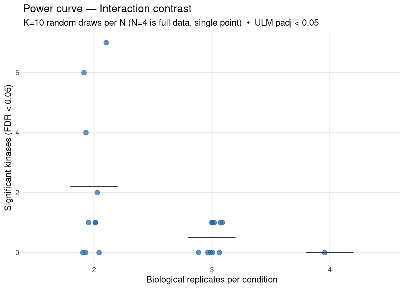
Empirical power curve for kinase activity inference on the APP × Microglia interaction contrast, built by subsampling the existing 4-replicates-per-condition data down to N ∈ {2, 3} reps per condition and re-running the full MSstatsPTM → decoupleR pipeline. Each subsample size is repeated K_DRAWS times with different random draws; N = 4 is the single reference point.
What this answers: “On the data I already have, how steeply does the number of significant kinases drop when I have fewer biological replicates per condition?” A steep drop from N=4→3→2 means more samples will help substantially. A flat curve means N=4 is already near saturation for this contrast (with this site coverage).
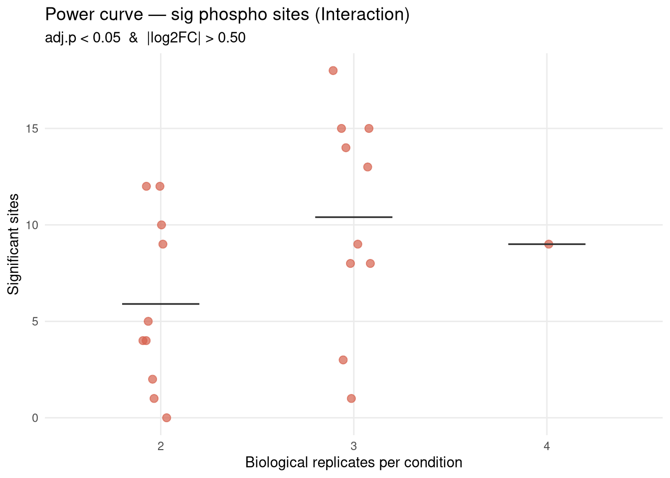
What this does NOT answer: how many new phospho sites would be detected with more samples. More mice typically rescue sites currently lost to feature drop-out — this analysis cannot model that, so its conclusions are a lower bound on the gain from increasing N. The site set used at every N here is whatever passes MSstatsPTM’s filters on that subset; sites that disappear at lower N reappear at N=4, but we can’t conjure sites that don’t exist at N=4.
base_dir <-"/nemo/lab/destrooperb/home/shared/zanettc/giulia_proteomics/phosphoproteomics"run_num <-"run3"results_dir <-file.path(base_dir, "results", run_num)objects_dir <-file.path(base_dir, "data", "processed", run_num)power_dir <-file.path(results_dir, "Power_downsampling")draws_dir <-file.path(objects_dir, "power_draws")dir.create(power_dir, recursive =TRUE, showWarnings =FALSE)dir.create(draws_dir, recursive =TRUE, showWarnings =FALSE)# Subsample sizes per condition (full = 4). Baseline N=4 is added automatically.N_VALUES <-c(2L, 3L)K_DRAWS <-10L # random draws per NSEED <-42LCONTRAST_NAME <-"Interaction_APP_x_Microglia"# Significance thresholds — match notebook 03 / 04SITE_PADJ_CUT <-0.05SITE_FC_CUT <-0.5KINASE_PADJ_CUT <-0.05# Parallel workers. Defaults to N=21 (the number of draws when K_DRAWS=10:# 1 + 10 + 10). Override via the SLURM_CPUS_PER_TASK env var so the same# notebook scales to whatever the SLURM job asks for. Clamped to n_draws.N_CORES <-as.integer(Sys.getenv("SLURM_CPUS_PER_TASK", "21"))# Paths needed by each worker. Workers re-load the cached input from disk# (rather than receiving 1.5+ GB tables via doSNOW serialisation) and# subset to their assigned runs before doing any work.PTM_INPUT_PATH <-file.path(objects_dir, "ptm_input.qs2")KS_NET_PATH <-file.path(objects_dir, "omnipath_kinase_substrate.qs2")
Load annotation
The full PTM + PROTEIN tables are NOT loaded in the parent process — each worker re-loads from PTM_INPUT_PATH and subsets to its kept runs immediately, to keep peak memory bounded.
Code
ann <-fread(file.path(objects_dir, "msstats_annotation.csv"))cat("Annotation:\n"); print(ann)
Every draw picks N BioReplicates from each of the four conditions (sampling without replacement), seeded for reproducibility. The full set (N = 4) is included once.
Pipeline function — one (N, draw) → kinase activities
Re-runs dataSummarizationPTM → groupComparisonPTM (Interaction contrast only) → decoupleR::run_ulm. Both PTM and PROTEIN are subsetted to the same kept runs so the protein-level adjustment is consistent.
Code
run_one_draw <-function(kept_runs, ann_full, ptm_input_path, ks_net_path, contrast_name, site_padj_cut, site_fc_cut, kinase_padj_cut) {# Pin BLAS/OMP threads to 1 inside the worker — env vars also set# this from the SLURM script, but belt-and-braces against thread# oversubscription when many workers run MSstatsPTM in parallel.try(RhpcBLASctl::blas_set_num_threads(1), silent =TRUE)try(RhpcBLASctl::omp_set_num_threads(1), silent =TRUE)# Worker reads the cached input itself so the 1.5+ GB tables are# not serialised through the doSNOW socket. Subset immediately, drop# the full object, and gc to keep peak memory bounded. ptm_input_full <- qs2::qs_read(ptm_input_path) ks_net <- qs2::qs_read(ks_net_path) ptm_sub <-as.data.table(ptm_input_full$PTM )[Run %in% kept_runs] prot_sub <-as.data.table(ptm_input_full$PROTEIN)[Run %in% kept_runs]rm(ptm_input_full); gc(verbose =FALSE) ann_sub <- ann_full[Run %in% kept_runs] ptm_input_sub <-list(PTM =as.data.frame(ptm_sub),PROTEIN =as.data.frame(prot_sub) ) summ <-suppressWarnings(dataSummarizationPTM(data = ptm_input_sub,normalization ="equalizeMedians",summaryMethod ="TMP",censoredInt ="NA",MBimpute =TRUE,featureSubset ="highQuality",remove_uninformative_feature_outlier =TRUE )) cond_levels <-levels(summ$PTM$ProteinLevelData$GROUP)stopifnot(all(c("hApp","hAppNLGF","hApp_FIRE","hAppNLGF_FIRE") %in% cond_levels))# Interaction-only contrast row w <-setNames(rep(0, length(cond_levels)), cond_levels) w[c("hApp","hAppNLGF","hApp_FIRE","hAppNLGF_FIRE")] <-c(-1, 1, 1, -1) cm <-matrix(w, nrow =1, dimnames =list(contrast_name, cond_levels)) res <-suppressWarnings(groupComparisonPTM(data = summ,contrast.matrix = cm,data.type ="LabelFree" )) adj <-as.data.table(res$ADJUSTED.Model)# Map site IDs the same way as notebook 04 adj[, Accession :=str_extract(Protein, "^[^_;]+")] adj[, Sites_in_id :=str_extract(Protein, "(?<=_)[STY][0-9]+(?:_[STY][0-9]+)*")] adj[, Gene :=mapIds(org.Mm.eg.db, keys = Accession,column ="SYMBOL", keytype ="UNIPROT",multiVals ="first")] adj[, Gene :=ifelse(is.na(Gene) | Gene =="", Accession, Gene)] sites_long <- adj[!is.na(Sites_in_id) &!is.na(Gene) &!is.na(Tvalue), .(Site =unlist(strsplit(Sites_in_id, "_"))), by = .(Label, Gene, log2FC, pvalue, adj.pvalue, Tvalue) ][, ID :=paste0(Gene, "_", Site)]# Build the t-stat matrix (one column: this contrast) mat <- sites_long[, .(stat =max(Tvalue, na.rm =TRUE)), by = .(ID, Label)] %>% tidyr::pivot_wider(id_cols = ID, names_from = Label,values_from = stat, values_fill =0) %>%as.data.frame()rownames(mat) <- mat$ID; mat$ID <-NULL mat <-as.matrix(mat) mat <- mat[rownames(mat) %in% ks_net$target, , drop =FALSE] mat <- mat[apply(mat, 1, function(x) all(is.finite(x))), , drop =FALSE] acts_ulm <- decoupleR::run_ulm(mat = mat, network = ks_net,.source ="source", .target ="target",.mor ="mor", minsize =5 ) ulm_tidy <- acts_ulm %>% dplyr::filter(statistic =="ulm") %>% dplyr::mutate(padj =p.adjust(p_value, method ="BH")) %>% dplyr::rename(Kinase = source, Activity = score) %>% dplyr::select(Kinase, Activity, p_value, padj) %>%as.data.table()# Summary scalars n_sig_sites <- adj[adj.pvalue < site_padj_cut &abs(log2FC) > site_fc_cut, .N] sig_kin <- ulm_tidy[padj < kinase_padj_cut][order(padj)]list(adj = adj,ulm_tidy = ulm_tidy,n_sig_sites = n_sig_sites,n_sig_kinases =nrow(sig_kin),sig_kinases = sig_kin$Kinase )}
Run all draws in parallel (resumable)
Each draw is cached at data/processed/run3/power_draws/draw_N{N}_d{draw_id}.qs2. The block below:
Filters draw_plan to draws without a cached result.
If all draws are cached (e.g. when rendering the Quarto HTML after a SLURM compute job), skips the cluster entirely.
Otherwise spins up min(N_CORES, n_uncached)doSNOW workers, each of which loads ptm_input.qs2 from disk itself and subsets to its kept runs before running MSstatsPTM. .errorhandling = "pass" lets the loop survive a single draw failure (e.g. degenerate N=2 design).
Code
to_run <- draw_plan[!file.exists(file)]if (nrow(to_run) ==0) {cat("All draws cached — skipping cluster setup.\n")} else { n_workers <-min(N_CORES, nrow(to_run))cat(sprintf("Spinning up %d worker(s) for %d uncached draw(s)...\n", n_workers, nrow(to_run)))# outfile = "" streams worker stdout/stderr to the parent process so# SLURM logs capture per-draw progress lines. cl <- parallel::makeCluster(n_workers, type ="SOCK", outfile ="") doSNOW::registerDoSNOW(cl)on.exit(try(parallel::stopCluster(cl), silent =TRUE), add =TRUE) WORKER_PACKAGES <-c("data.table", "qs2", "MSstats", "MSstatsPTM", "decoupleR","dplyr", "tidyr", "stringr", "AnnotationDbi", "org.Mm.eg.db","RhpcBLASctl" ) results <-foreach(i =seq_len(nrow(to_run)),.packages = WORKER_PACKAGES,.export =c("run_one_draw", "ann", "to_run","PTM_INPUT_PATH", "KS_NET_PATH","CONTRAST_NAME","SITE_PADJ_CUT", "SITE_FC_CUT", "KINASE_PADJ_CUT"),.errorhandling ="pass" ) %dopar% { kept <-strsplit(to_run$runs_csv[i], ",")[[1]] t0 <-Sys.time() out <-run_one_draw(kept_runs = kept,ann_full = ann,ptm_input_path = PTM_INPUT_PATH,ks_net_path = KS_NET_PATH,contrast_name = CONTRAST_NAME,site_padj_cut = SITE_PADJ_CUT,site_fc_cut = SITE_FC_CUT,kinase_padj_cut = KINASE_PADJ_CUT ) out$meta <-list(N = to_run$N[i],draw_id = to_run$draw_id[i],seed = to_run$seed[i],runs = kept,elapsed =as.numeric(difftime(Sys.time(), t0, units ="secs")) ) qs2::qs_save(out, to_run$file[i])cat(sprintf("[worker pid=%d] N=%d draw=%d → %d sig sites, %d sig kinases (%.1f min)\n",Sys.getpid(), to_run$N[i], to_run$draw_id[i], out$n_sig_sites, out$n_sig_kinases, out$meta$elapsed /60))data.table(N = to_run$N[i],draw_id = to_run$draw_id[i],n_sig_sites = out$n_sig_sites,n_sig_kinases = out$n_sig_kinases,elapsed_min = out$meta$elapsed /60,status ="ok" ) } parallel::stopCluster(cl)# Report any iterations that came back as error objects (errorhandling=pass). bad <-which(vapply(results, inherits, logical(1), what ="error"))if (length(bad)) {cat(sprintf("\n%d draw(s) failed; their cache files will be missing:\n",length(bad)))for (k in bad) {cat(sprintf(" - draw row %d: %s\n", k, conditionMessage(results[[k]]))) } }}
For each kinase, count how often it reaches FDR < 0.05 across the K draws at each N. Kinases that are robustly significant at low N are the “easy wins”; kinases that appear only at N=4 are the ones losing power from sample size.
Mean curve still rising at N=4 → more mice will likely raise the kinase count. Magnitude of expected gain is bounded by the slope here (and is in fact larger, because more N also detects new sites).
Mean curve plateauing at N=4 → either the contrast is genuinely null beyond a small set of strong kinases, or the bottleneck is site coverage (not N). In that case, switching to a deeper acquisition or relaxing site-level filters may help more than adding mice.
High variance across draws at N=2 or N=3 → indicates fragile inference. Look at kinase_persistence.csv to see which kinases come and go between draws vs. which are stable.
Source Code
---title: "7. Power downsampling — Interaction contrast"---## OverviewEmpirical power curve for kinase activity inference on the APP × Microglia interaction contrast, built by subsampling the existing 4-replicates-per-condition data down to N ∈ {2, 3} reps per condition and re-running the full MSstatsPTM → decoupleR pipeline. Each subsample size is repeated `K_DRAWS` times with different random draws; N = 4 is the single reference point.**What this answers:** "On the data I already have, how steeply does the number of significant kinases drop when I have fewer biological replicates per condition?" A steep drop from N=4→3→2 means more samples will help substantially. A flat curve means N=4 is already near saturation for this contrast (with this site coverage).**What this does NOT answer:** how many *new* phospho sites would be detected with more samples. More mice typically rescue sites currently lost to feature drop-out — this analysis cannot model that, so its conclusions are a **lower bound** on the gain from increasing N. The site set used at every N here is whatever passes MSstatsPTM's filters on that subset; sites that disappear at lower N reappear at N=4, but we can't conjure sites that don't exist at N=4.**Inputs (from run3 of notebook 02 + 04):**- `ptm_input.qs2` — paired PTM + PROTEIN feature-level input (post-localisation + Q-value filter)- `msstats_annotation.csv` — Run / Condition / BioReplicate mapping- `omnipath_kinase_substrate.qs2` — mouse kinase–substrate network## Libraries```{r setup, include=FALSE, message=FALSE}library(data.table)library(qs2)library(MSstats)library(MSstatsPTM)library(decoupleR)library(dplyr)library(tidyr)library(stringr)library(ggplot2)library(AnnotationDbi)library(org.Mm.eg.db)library(foreach)library(doSNOW)library(parallel)library(RhpcBLASctl)```## Directories and parameters```{r}base_dir <-"/nemo/lab/destrooperb/home/shared/zanettc/giulia_proteomics/phosphoproteomics"run_num <-"run3"results_dir <-file.path(base_dir, "results", run_num)objects_dir <-file.path(base_dir, "data", "processed", run_num)power_dir <-file.path(results_dir, "Power_downsampling")draws_dir <-file.path(objects_dir, "power_draws")dir.create(power_dir, recursive =TRUE, showWarnings =FALSE)dir.create(draws_dir, recursive =TRUE, showWarnings =FALSE)# Subsample sizes per condition (full = 4). Baseline N=4 is added automatically.N_VALUES <-c(2L, 3L)K_DRAWS <-10L # random draws per NSEED <-42LCONTRAST_NAME <-"Interaction_APP_x_Microglia"# Significance thresholds — match notebook 03 / 04SITE_PADJ_CUT <-0.05SITE_FC_CUT <-0.5KINASE_PADJ_CUT <-0.05# Parallel workers. Defaults to N=21 (the number of draws when K_DRAWS=10:# 1 + 10 + 10). Override via the SLURM_CPUS_PER_TASK env var so the same# notebook scales to whatever the SLURM job asks for. Clamped to n_draws.N_CORES <-as.integer(Sys.getenv("SLURM_CPUS_PER_TASK", "21"))# Paths needed by each worker. Workers re-load the cached input from disk# (rather than receiving 1.5+ GB tables via doSNOW serialisation) and# subset to their assigned runs before doing any work.PTM_INPUT_PATH <-file.path(objects_dir, "ptm_input.qs2")KS_NET_PATH <-file.path(objects_dir, "omnipath_kinase_substrate.qs2")```## Load annotationThe full PTM + PROTEIN tables are NOT loaded in the parent process — each worker re-loads from `PTM_INPUT_PATH` and subsets to its kept runs immediately, to keep peak memory bounded.```{r load}ann <- fread(file.path(objects_dir, "msstats_annotation.csv"))cat("Annotation:\n"); print(ann)```## Build draw planEvery draw picks `N` BioReplicates from each of the four conditions (sampling without replacement), seeded for reproducibility. The full set (N = 4) is included once.```{r draw_plan}set.seed(SEED)conds <- unique(ann$Condition)make_draw <- function(N, seed) { set.seed(seed) do.call(c, lapply(conds, function(co) { runs_co <- ann[Condition == co, Run] sample(runs_co, N) }))}draw_plan <- rbindlist(lapply(N_VALUES, function(N) { data.table( N = N, draw_id = seq_len(K_DRAWS), seed = SEED + 1000L * N + seq_len(K_DRAWS), runs_csv = vapply(seq_len(K_DRAWS), function(k) paste(make_draw(N, SEED + 1000L * N + k), collapse = ","), character(1)) )}))# Add the N=4 baseline (no random subset — all 16 samples)draw_plan <- rbindlist(list( data.table(N = 4L, draw_id = 0L, seed = NA_integer_, runs_csv = paste(ann$Run, collapse = ",")), draw_plan), use.names = TRUE)draw_plan[, file := file.path(draws_dir, sprintf("draw_N%d_d%02d.qs2", N, draw_id))]print(draw_plan[, .(N, draw_id, seed, n_runs = lengths(strsplit(runs_csv, ",")))])```## Pipeline function — one (N, draw) → kinase activitiesRe-runs `dataSummarizationPTM` → `groupComparisonPTM` (Interaction contrast only) → `decoupleR::run_ulm`. Both PTM and PROTEIN are subsetted to the same kept runs so the protein-level adjustment is consistent.```{r pipeline_fn}run_one_draw <- function(kept_runs, ann_full, ptm_input_path, ks_net_path, contrast_name, site_padj_cut, site_fc_cut, kinase_padj_cut) { # Pin BLAS/OMP threads to 1 inside the worker — env vars also set # this from the SLURM script, but belt-and-braces against thread # oversubscription when many workers run MSstatsPTM in parallel. try(RhpcBLASctl::blas_set_num_threads(1), silent = TRUE) try(RhpcBLASctl::omp_set_num_threads(1), silent = TRUE) # Worker reads the cached input itself so the 1.5+ GB tables are # not serialised through the doSNOW socket. Subset immediately, drop # the full object, and gc to keep peak memory bounded. ptm_input_full <- qs2::qs_read(ptm_input_path) ks_net <- qs2::qs_read(ks_net_path) ptm_sub <- as.data.table(ptm_input_full$PTM )[Run %in% kept_runs] prot_sub <- as.data.table(ptm_input_full$PROTEIN)[Run %in% kept_runs] rm(ptm_input_full); gc(verbose = FALSE) ann_sub <- ann_full[Run %in% kept_runs] ptm_input_sub <- list( PTM = as.data.frame(ptm_sub), PROTEIN = as.data.frame(prot_sub) ) summ <- suppressWarnings(dataSummarizationPTM( data = ptm_input_sub, normalization = "equalizeMedians", summaryMethod = "TMP", censoredInt = "NA", MBimpute = TRUE, featureSubset = "highQuality", remove_uninformative_feature_outlier = TRUE )) cond_levels <- levels(summ$PTM$ProteinLevelData$GROUP) stopifnot(all(c("hApp","hAppNLGF","hApp_FIRE","hAppNLGF_FIRE") %in% cond_levels)) # Interaction-only contrast row w <- setNames(rep(0, length(cond_levels)), cond_levels) w[c("hApp","hAppNLGF","hApp_FIRE","hAppNLGF_FIRE")] <- c(-1, 1, 1, -1) cm <- matrix(w, nrow = 1, dimnames = list(contrast_name, cond_levels)) res <- suppressWarnings(groupComparisonPTM( data = summ, contrast.matrix = cm, data.type = "LabelFree" )) adj <- as.data.table(res$ADJUSTED.Model) # Map site IDs the same way as notebook 04 adj[, Accession := str_extract(Protein, "^[^_;]+")] adj[, Sites_in_id := str_extract(Protein, "(?<=_)[STY][0-9]+(?:_[STY][0-9]+)*")] adj[, Gene := mapIds(org.Mm.eg.db, keys = Accession, column = "SYMBOL", keytype = "UNIPROT", multiVals = "first")] adj[, Gene := ifelse(is.na(Gene) | Gene == "", Accession, Gene)] sites_long <- adj[!is.na(Sites_in_id) & !is.na(Gene) & !is.na(Tvalue), .(Site = unlist(strsplit(Sites_in_id, "_"))), by = .(Label, Gene, log2FC, pvalue, adj.pvalue, Tvalue) ][, ID := paste0(Gene, "_", Site)] # Build the t-stat matrix (one column: this contrast) mat <- sites_long[, .(stat = max(Tvalue, na.rm = TRUE)), by = .(ID, Label)] %>% tidyr::pivot_wider(id_cols = ID, names_from = Label, values_from = stat, values_fill = 0) %>% as.data.frame() rownames(mat) <- mat$ID; mat$ID <- NULL mat <- as.matrix(mat) mat <- mat[rownames(mat) %in% ks_net$target, , drop = FALSE] mat <- mat[apply(mat, 1, function(x) all(is.finite(x))), , drop = FALSE] acts_ulm <- decoupleR::run_ulm( mat = mat, network = ks_net, .source = "source", .target = "target", .mor = "mor", minsize = 5 ) ulm_tidy <- acts_ulm %>% dplyr::filter(statistic == "ulm") %>% dplyr::mutate(padj = p.adjust(p_value, method = "BH")) %>% dplyr::rename(Kinase = source, Activity = score) %>% dplyr::select(Kinase, Activity, p_value, padj) %>% as.data.table() # Summary scalars n_sig_sites <- adj[adj.pvalue < site_padj_cut & abs(log2FC) > site_fc_cut, .N] sig_kin <- ulm_tidy[padj < kinase_padj_cut][order(padj)] list( adj = adj, ulm_tidy = ulm_tidy, n_sig_sites = n_sig_sites, n_sig_kinases = nrow(sig_kin), sig_kinases = sig_kin$Kinase )}```## Run all draws in parallel (resumable)Each draw is cached at `data/processed/run3/power_draws/draw_N{N}_d{draw_id}.qs2`. The block below:1. Filters `draw_plan` to draws without a cached result.2. If all draws are cached (e.g. when rendering the Quarto HTML after a SLURM compute job), skips the cluster entirely.3. Otherwise spins up `min(N_CORES, n_uncached)``doSNOW` workers, each of which loads `ptm_input.qs2` from disk itself and subsets to its kept runs before running MSstatsPTM. `.errorhandling = "pass"` lets the loop survive a single draw failure (e.g. degenerate N=2 design).```{r run_loop, message=FALSE}to_run <- draw_plan[!file.exists(file)]if (nrow(to_run) == 0) { cat("All draws cached — skipping cluster setup.\n")} else { n_workers <- min(N_CORES, nrow(to_run)) cat(sprintf("Spinning up %d worker(s) for %d uncached draw(s)...\n", n_workers, nrow(to_run))) # outfile = "" streams worker stdout/stderr to the parent process so # SLURM logs capture per-draw progress lines. cl <- parallel::makeCluster(n_workers, type = "SOCK", outfile = "") doSNOW::registerDoSNOW(cl) on.exit(try(parallel::stopCluster(cl), silent = TRUE), add = TRUE) WORKER_PACKAGES <- c( "data.table", "qs2", "MSstats", "MSstatsPTM", "decoupleR", "dplyr", "tidyr", "stringr", "AnnotationDbi", "org.Mm.eg.db", "RhpcBLASctl" ) results <- foreach( i = seq_len(nrow(to_run)), .packages = WORKER_PACKAGES, .export = c("run_one_draw", "ann", "to_run", "PTM_INPUT_PATH", "KS_NET_PATH", "CONTRAST_NAME", "SITE_PADJ_CUT", "SITE_FC_CUT", "KINASE_PADJ_CUT"), .errorhandling = "pass" ) %dopar% { kept <- strsplit(to_run$runs_csv[i], ",")[[1]] t0 <- Sys.time() out <- run_one_draw( kept_runs = kept, ann_full = ann, ptm_input_path = PTM_INPUT_PATH, ks_net_path = KS_NET_PATH, contrast_name = CONTRAST_NAME, site_padj_cut = SITE_PADJ_CUT, site_fc_cut = SITE_FC_CUT, kinase_padj_cut = KINASE_PADJ_CUT ) out$meta <- list( N = to_run$N[i], draw_id = to_run$draw_id[i], seed = to_run$seed[i], runs = kept, elapsed = as.numeric(difftime(Sys.time(), t0, units = "secs")) ) qs2::qs_save(out, to_run$file[i]) cat(sprintf("[worker pid=%d] N=%d draw=%d → %d sig sites, %d sig kinases (%.1f min)\n", Sys.getpid(), to_run$N[i], to_run$draw_id[i], out$n_sig_sites, out$n_sig_kinases, out$meta$elapsed / 60)) data.table( N = to_run$N[i], draw_id = to_run$draw_id[i], n_sig_sites = out$n_sig_sites, n_sig_kinases = out$n_sig_kinases, elapsed_min = out$meta$elapsed / 60, status = "ok" ) } parallel::stopCluster(cl) # Report any iterations that came back as error objects (errorhandling=pass). bad <- which(vapply(results, inherits, logical(1), what = "error")) if (length(bad)) { cat(sprintf("\n%d draw(s) failed; their cache files will be missing:\n", length(bad))) for (k in bad) { cat(sprintf(" - draw row %d: %s\n", k, conditionMessage(results[[k]]))) } }}```## Aggregate```{r aggregate}all_draws <- rbindlist(lapply(draw_plan$file, function(f) { x <- qs_read(f) data.table( N = x$meta$N, draw_id = x$meta$draw_id, n_sig_sites = x$n_sig_sites, n_sig_kinases = x$n_sig_kinases, sig_kinases = paste(x$sig_kinases, collapse = ", ") )}))all_draws[, N := factor(N, levels = sort(unique(N)))]print(all_draws[order(N, draw_id)])fwrite(all_draws, file.path(power_dir, "power_summary.csv"))```## Per-kinase persistence across drawsFor each kinase, count how often it reaches FDR < 0.05 across the K draws at each N. Kinases that are robustly significant at low N are the "easy wins"; kinases that appear only at N=4 are the ones losing power from sample size.```{r kinase_persistence}per_kin <- rbindlist(lapply(draw_plan$file, function(f) { x <- qs_read(f) if (length(x$sig_kinases) == 0) { return(data.table(N = integer(), draw_id = integer(), Kinase = character())) } data.table(N = x$meta$N, draw_id = x$meta$draw_id, Kinase = x$sig_kinases)}))n_per_N <- draw_plan[, .(n_draws = uniqueN(draw_id)), by = N]if (nrow(per_kin) > 0) { persistence <- per_kin[, .(n_hit = .N), by = .(N, Kinase)] persistence <- merge(persistence, n_per_N, by = "N") persistence[, hit_rate := n_hit / n_draws] persistence <- persistence[order(N, -hit_rate, Kinase)]} else { persistence <- data.table(N = integer(), Kinase = character(), n_hit = integer(), n_draws = integer(), hit_rate = numeric())}print(persistence)fwrite(persistence, file.path(power_dir, "kinase_persistence.csv"))```## Plot — power curve```{r plot_power, fig.width=7, fig.height=5}p <- ggplot(all_draws, aes(x = N, y = n_sig_kinases)) + geom_jitter(width = 0.12, height = 0, size = 2.5, alpha = 0.7, colour = "#2166AC") + stat_summary(fun = mean, geom = "crossbar", width = 0.4, colour = "grey20", fatten = 1.2) + labs( title = "Power curve — Interaction contrast", subtitle = sprintf( "K=%d random draws per N (N=4 is full data, single point) • ULM padj < %.2f", K_DRAWS, KINASE_PADJ_CUT), x = "Biological replicates per condition", y = "Significant kinases (FDR < 0.05)" ) + theme_minimal(base_size = 11) + theme(panel.grid.minor = element_blank())print(p)ggsave(file.path(power_dir, "power_curve_kinases.pdf"), p, width = 7, height = 5, device = cairo_pdf)p_sites <- ggplot(all_draws, aes(x = N, y = n_sig_sites)) + geom_jitter(width = 0.12, height = 0, size = 2.5, alpha = 0.7, colour = "#D6604D") + stat_summary(fun = mean, geom = "crossbar", width = 0.4, colour = "grey20", fatten = 1.2) + labs( title = "Power curve — sig phospho sites (Interaction)", subtitle = sprintf("adj.p < %.2f & |log2FC| > %.2f", SITE_PADJ_CUT, SITE_FC_CUT), x = "Biological replicates per condition", y = "Significant sites" ) + theme_minimal(base_size = 11) + theme(panel.grid.minor = element_blank())print(p_sites)ggsave(file.path(power_dir, "power_curve_sites.pdf"), p_sites, width = 7, height = 5, device = cairo_pdf)```## Interpretation cues- **Mean curve still rising at N=4** → more mice will likely raise the kinase count. Magnitude of expected gain is bounded by the slope here (and is in fact larger, because more N also detects new sites).- **Mean curve plateauing at N=4** → either the contrast is genuinely null beyond a small set of strong kinases, or the bottleneck is site coverage (not N). In that case, switching to a deeper acquisition or relaxing site-level filters may help more than adding mice.- **High variance across draws at N=2 or N=3** → indicates fragile inference. Look at `kinase_persistence.csv` to see which kinases come and go between draws vs. which are stable.