4. GSEA

==================================================================

GSEA for proteomics data

This script performs GSEA on the MSstats differential-abundance results for the Giulia mouse microglia proteome (hApp / hAppNLGF / hApp_FIRE / hAppNLGF_FIRE). It uses the fgsea package.

Workflow overview

1. Data Loading: Imports the MSstats group-comparison table (CSV) from notebook 02a.

2. Gene Set Prep: Loads mouse pathways from msigdbr (GO / KEGG / cell-type C8).

3. Ranking: Ranks proteins by Log2FC for every contrast.

4. Analysis Loop: Runs GSEA for every combination of [Comparison x Gene Set Database].

5. Visualization:

Generates summary bar plots of top 10 and bottom 10 NES.

Generates specific enrichment plots (mountain plots) for key pathways of choice.

==================================================================

Load libraries

Code

library(data.table)
library(qs2)
library(ggrepel)
library(ggplot2)
library(stringr)
library(glue)
library(dplyr)
library(msigdbr)
library(fgsea)
library(viridis)
library(readxl)

Set directories

Code

base_dir <- "/nemo/lab/destrooperb/home/shared/zanettc/giulia_proteomics/bulk_proteomics"
run_num  <- "run4"

results_dir <- file.path(base_dir, "results", run_num)
objects_dir <- file.path(base_dir, "data", "processed", run_num)
input_dir   <- file.path(base_dir, "input")

dir.create(results_dir, recursive = TRUE, showWarnings = FALSE)
dir.create(objects_dir, recursive = TRUE, showWarnings = FALSE)

Read in DE data

Code

#seurat <- qs_read(glue("output/{run_num}/objects/prelabelled_integrated_rpca.qs2"))
res_df <- fread(file.path(results_dir, "Full_GroupComparison_Results.csv"))
clean_spec_raw <- fread(file.path(base_dir, "data/processed/run1/clean_spec_raw.csv"))

protein_dictionary <- fread(file.path(objects_dir, 'protein_dictionary.csv'))

Define helper functions

Code

# ==============================================================================
# 1. HELPER FUNCTIONS
# ==============================================================================

# A. Create Rank Vector from MSstats Data
prep_msstats_ranks <- function(msstats_res, dict, comp_label) {
  df <- msstats_res %>%
    filter(Label == comp_label) %>%
    # Keep only finite log2FC values (removes Inf and -Inf)
    filter(is.finite(log2FC)) %>%
    left_join(dict, by = "Protein") %>%
    filter(!is.na(Gene) & Gene != "") %>%
    mutate(Gene = toupper(Gene)) %>%
    mutate(adj.pvalue = ifelse(adj.pvalue == 0, 1e-300, adj.pvalue)) %>%
    group_by(Gene) %>%
    slice_max(order_by = abs(log2FC), n = 1, with_ties = FALSE) %>%
    ungroup()
  
  #rank by logFC
  ranks <- df$log2FC
  names(ranks) <- df$Gene
  
  # Remove any unexpected NAs in names or values
  ranks <- ranks[!is.na(ranks) & !is.na(names(ranks))]
  
  return(sort(ranks, decreasing = TRUE))
}

# B. Core GSEA & Plotting Function
run_gsea_analysis <- function(ranks, 
                              comparison_name, 
                              geneset_name,    
                              pathways, 
                              base_objects_dir, 
                              base_graphs_dir,  
                              color_A = "firebrick3",
                              color_B = "navy") {
  
  message(glue("Running GSEA | Set: {geneset_name} | Comp: {comparison_name}"))
  
  # --- DYNAMIC LABEL GENERATION ---
  # Split the comparison name to get the two groups (e.g., "PlaqueNear" and "PlaqueFar")
  comp_parts <- str_split(comparison_name, "_vs_")[[1]]
  if(length(comp_parts) == 2) {
    group_A_label <- glue("{comp_parts[1]} Enriched") # Positive NES
    group_B_label <- glue("{comp_parts[2]} Enriched") # Negative NES
  } else {
    group_A_label <- "Group A Enriched"
    group_B_label <- "Group B Enriched"
  }
  
  # Clean title for the plot
  clean_comp_title <- gsub("_", " ", comparison_name)
  plot_title <- glue("{clean_comp_title} ({geneset_name})")

  # --- Directories ---
  current_objects_dir <- file.path(base_objects_dir, "GSEA_Analysis", comparison_name)
  current_graphs_dir  <- file.path(base_graphs_dir, "GSEA_Analysis", comparison_name)
  dir.create(current_objects_dir, recursive = TRUE, showWarnings = FALSE)
  dir.create(current_graphs_dir, recursive = TRUE, showWarnings = FALSE)
  
  # --- Run FGSEA ---
  pathways_upper <- lapply(pathways, toupper)
  set.seed(42)
  fgsea_res <- fgsea(
    pathways = pathways_upper,
    stats    = ranks,
    minSize  = 15,
    maxSize  = 3000,
    nPermSimple = 10000,
    BPPARAM  = BiocParallel::MulticoreParam(workers = 4, progressbar = FALSE)
  )
  
  if (nrow(fgsea_res) == 0) {
    warning(glue("No significant pathways for {geneset_name} in {comparison_name}"))
    return(NULL)
  }
  
  # --- Tidy & Save ---
  fgsea_res_tidy <- fgsea_res %>%
    as_tibble() %>%
    mutate(leadingEdge = sapply(leadingEdge, paste, collapse = ",")) %>%
    mutate(pathway = gsub("_geneset", "", pathway)) %>% 
    arrange(padj)
  
  write.csv(fgsea_res_tidy, file.path(current_objects_dir, glue("Table_{geneset_name}.csv")), row.names = FALSE)
  
  # --- Barplot ---
  top_gsea <- fgsea_res_tidy %>%
    arrange(desc(NES)) %>%
    slice_head(n = 10) %>%
    bind_rows(fgsea_res_tidy %>% arrange(NES) %>% slice_head(n = 10)) %>%
    distinct(pathway, .keep_all = TRUE) %>%
    mutate(
      sig_label = case_when(
        padj < 0.001 ~ "***",
        padj < 0.01  ~ "**",
        padj < 0.05  ~ "*",
        TRUE         ~ ""
      ),
      # Apply dynamic labels based on NES direction
      fill_group = ifelse(NES > 0, group_A_label, group_B_label),
      pathway = factor(pathway, levels = unique(pathway[order(NES)]))
    )
  
  if (nrow(top_gsea) == 0) return(fgsea_res_tidy)
  
  axis_zoom <- 3.5 
  
  p_bar <- ggplot(top_gsea, aes(x = NES, y = pathway, fill = fill_group)) +
    geom_col(width = 0.7) +
    geom_text(aes(label = sig_label, hjust = ifelse(NES > 0, 1.2, -0.2)), 
              color = "white", size = 5, vjust = 0.75, fontface = "bold") +
    scale_fill_manual(values = setNames(c(color_A, color_B), c(group_A_label, group_B_label))) +
    scale_x_continuous(breaks = seq(-axis_zoom, axis_zoom, 0.5),
                       labels = function(x) ifelse(x %% 1 == 0, x, "")) + 
    labs(x = "Normalized Enrichment Score (NES)", y = NULL, title = plot_title) +
    theme_bw(base_size = 14) +
    theme(
      panel.grid.major.x = element_line(color = "grey92", linewidth = 0.5),
      panel.grid.major.y = element_blank(),
      panel.grid.minor   = element_blank(),
      panel.border = element_rect(colour = "black", fill = NA, linewidth = 1.5),
      legend.position = "none",
      plot.title = element_text(hjust = 0.5, face = "bold", size = 16, margin = margin(b = 40)),
      plot.margin = margin(t = 40, r = 20, b = 20, l = 20, unit = "pt"),
      #ensure y axis has enough room, and tightens lines together
      axis.text.y = element_text(size = 9, lineheight = 0.8)
    ) +
    scale_y_discrete(labels = function(x) str_wrap(gsub("_", " ", x), width = 50)) +
    # Dynamic text annotations at the top of the plot
    annotate("text", x = -axis_zoom/2, y = Inf, 
             label = glue("^ {group_B_label}"), color = color_B, size = 5, fontface = "bold", vjust = -1.0) +
    annotate("text", x = axis_zoom/2, y = Inf, 
             label = glue("^ {group_A_label}"), color = color_A, size = 5, fontface = "bold", vjust = -1.0) +
    coord_cartesian(xlim = c(-axis_zoom, axis_zoom), clip = "off")
  
  dyn_h <- 2 + (nrow(top_gsea) * 0.3)
  dyn_w <- 5 + (max(nchar(as.character(top_gsea$pathway))) * 0.12)
  
  print(p_bar)
  
  ggsave(filename = file.path(current_graphs_dir, glue("Barplot_{geneset_name}.pdf")), 
         plot = p_bar, width = dyn_w, height = dyn_h, limitsize = FALSE)
  
  # --- Dotplot (Top 10 Highest NES) ---
  top_nes_gsea <- fgsea_res_tidy %>%
    arrange(desc(NES)) %>%   
    slice_head(n = 10) %>%   
    mutate(pathway = factor(pathway, levels = unique(pathway[order(NES)])))

  if (nrow(top_nes_gsea) > 0) {
    # Define our wrap width
    wrap_width <- 45
    
    p_sig <- ggplot(top_nes_gsea, aes(x = NES, y = pathway, color = NES, size = -log10(padj))) +
      geom_vline(xintercept = 0, linetype = "dashed", color = "grey60") +
      geom_point(alpha = 0.8) +
      scale_color_gradient2(low = color_B, mid = "grey90", high = color_A, midpoint = 0, name = "NES") +
      scale_size_continuous(range = c(3, 8), name = "-log10(padj)") +
      labs(x = "Normalized Enrichment Score (NES)", y = NULL, 
           title = glue("Top 10 Highest NES:\n{clean_comp_title} ({geneset_name})")) +
      theme_bw(base_size = 14) +
      theme(
        panel.grid.major.x = element_line(color = "grey92", linewidth = 0.5),
        panel.grid.major.y = element_line(color = "grey92", linewidth = 0.5, linetype = "dotted"),
        panel.grid.minor   = element_blank(),
        panel.border = element_rect(colour = "black", fill = NA, linewidth = 1.5),
        plot.title = element_text(hjust = 0.5, face = "bold", size = 14, margin = margin(b = 20)),
        plot.margin = margin(t = 20, r = 10, b = 10, l = 10, unit = "pt"),
        axis.text.y = element_text(lineheight = 0.8) 
      ) +
      scale_y_discrete(labels = function(x) str_wrap(gsub("_", " ", x), width = wrap_width))

    # --- DYNAMIC SIZING ---
    # Cap the character count at wrap_width so the plot doesn't stretch endlessly horizontally
    max_chars <- min(max(nchar(as.character(top_nes_gsea$pathway))), wrap_width)
    
    # Calculate dimensions: enough base room for the plot/legends + scaled room for text/points
    dyn_h_sig <- 3 + (nrow(top_nes_gsea) * 0.4)
    dyn_w_sig <- 4.5 + (max_chars * 0.1) 
    
    ggsave(filename = file.path(current_graphs_dir, glue("Dotplot_Top10_NES_{geneset_name}.pdf")), 
           plot = p_sig, width = dyn_w_sig, height = dyn_h_sig, limitsize = FALSE)
  }
  
  
  return(fgsea_res_tidy)
}

Load data

Code

# ==============================================================================
# 2. CONFIG & DATA LOADING
# ==============================================================================

GLOBAL_CONFIG <- list(
  output_dir = file.path(results_dir, "GSEA_Results_Master"), 
  group_A    = "",
  group_B    = "",
  col_A      = "firebrick3",
  col_B      = "navy"
)

# Load Gene Sets (Mus musculus)

#GO (C5: GOBP/GOCC/GOMF) + KEGG (C2: CP:KEGG_MEDICUS)
go_df <- msigdbr(species = "Mus musculus", collection = "C5", subcollection = "GO:BP")
go_list <- split(x = go_df$gene_symbol, f = go_df$gs_name)
kegg_df <- msigdbr(species = "Mus musculus", collection = "C2", subcollection = "CP:KEGG_MEDICUS")
kegg_list <- split(x = kegg_df$gene_symbol, f = kegg_df$gs_name)
go_kegg_list <- c(go_list, kegg_list)

#cell type signature sets
c8_df <- msigdbr(species = "Mus musculus", collection = "C8")
c8_list <- split(x = c8_df$gene_symbol, f = c8_df$gs_name)


# Create master list
gene_sets_master <- list(
  "GO_KEGG" = go_kegg_list,
  "cell_type_sigs_c8" = c8_list
)

#Create Rank Vectors directly from MSstats output
comparisons_master <- list(
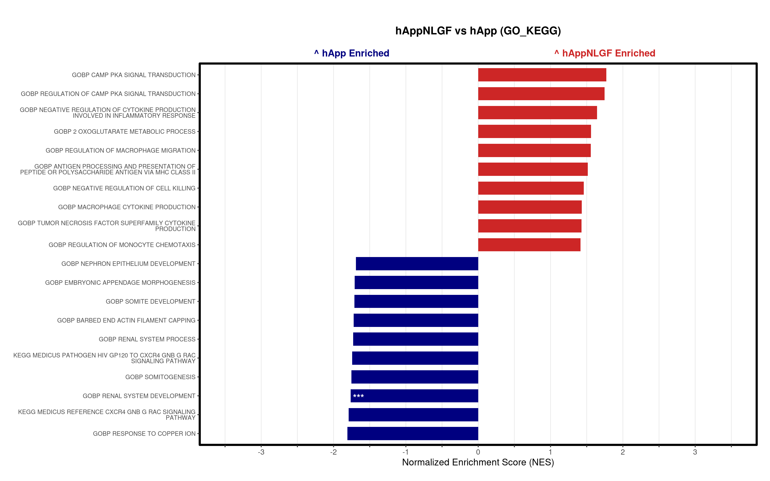
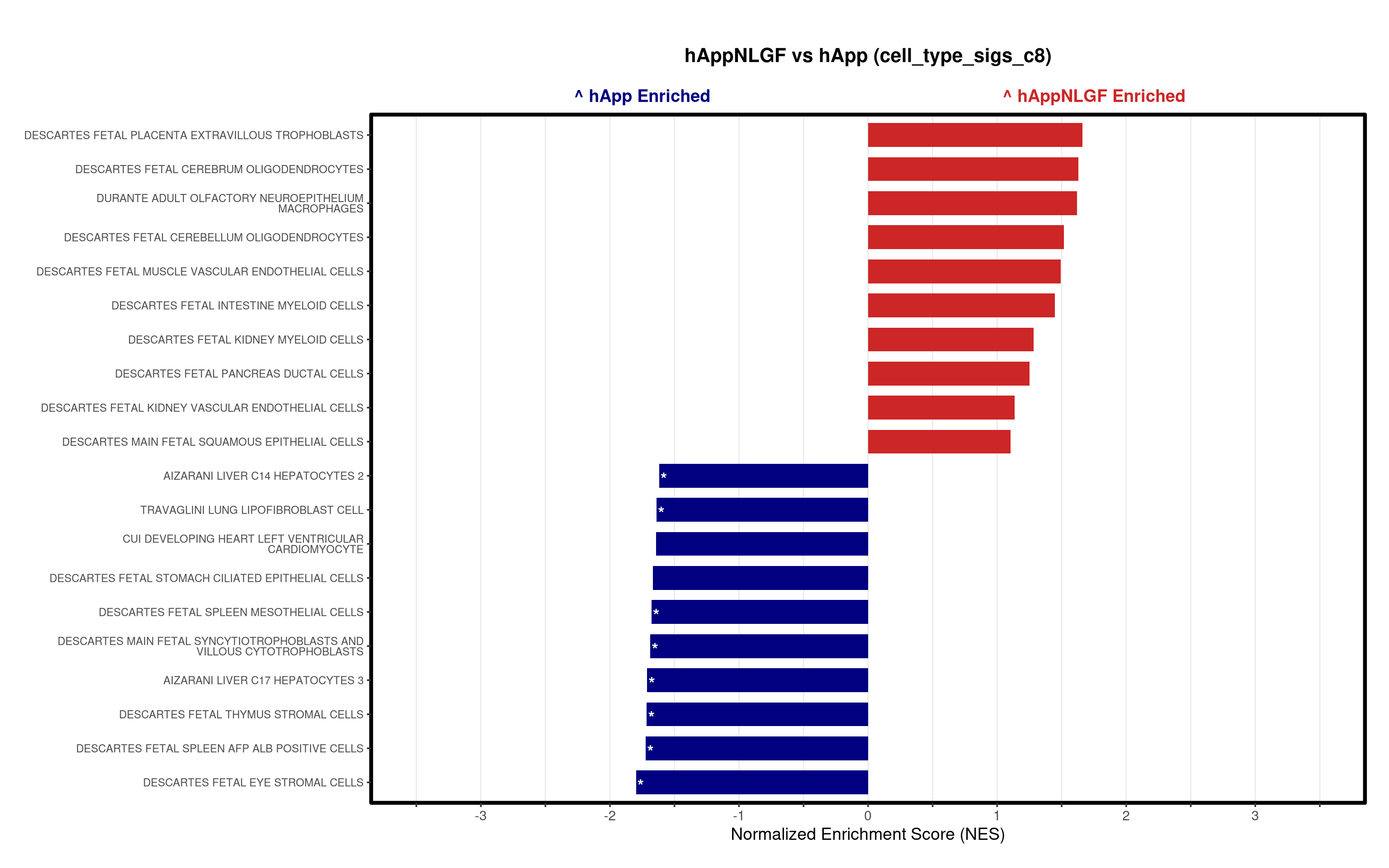
  "hAppNLGF_vs_hApp"            = prep_msstats_ranks(res_df, protein_dictionary, "hAppNLGF_vs_hApp"),
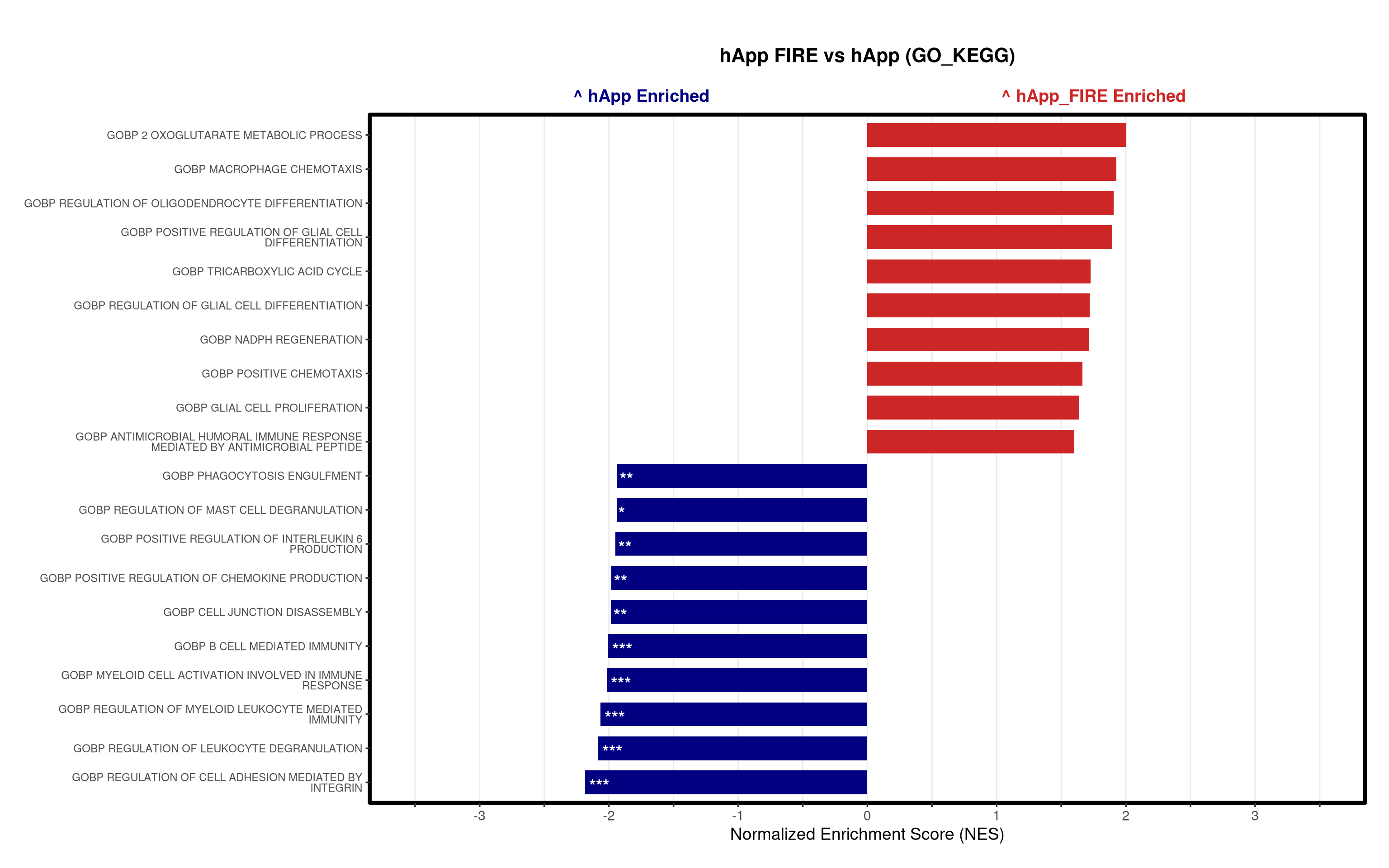
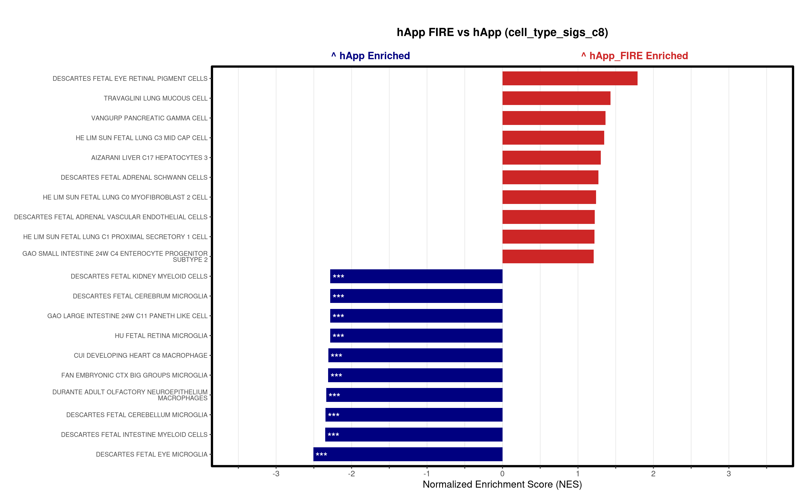
  "hApp_FIRE_vs_hApp"           = prep_msstats_ranks(res_df, protein_dictionary, "hApp_FIRE_vs_hApp"),
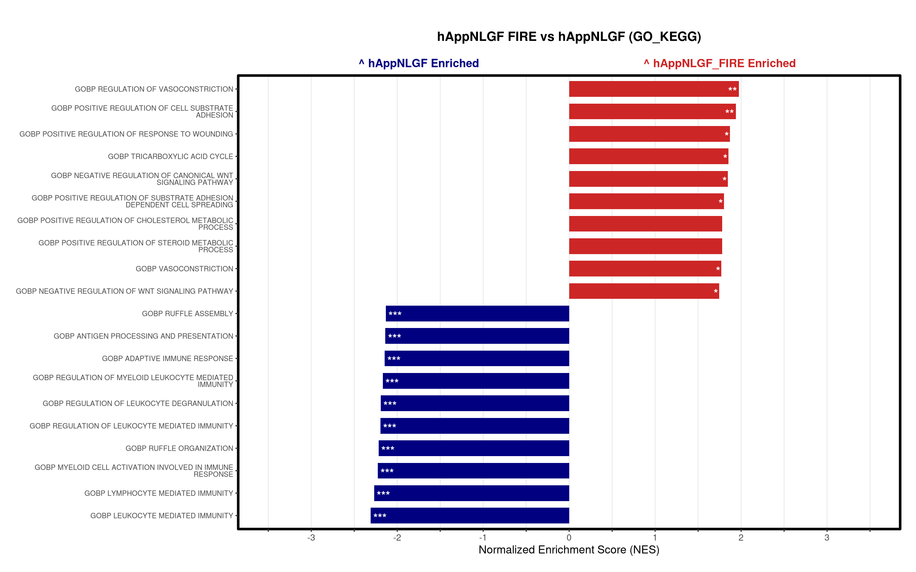
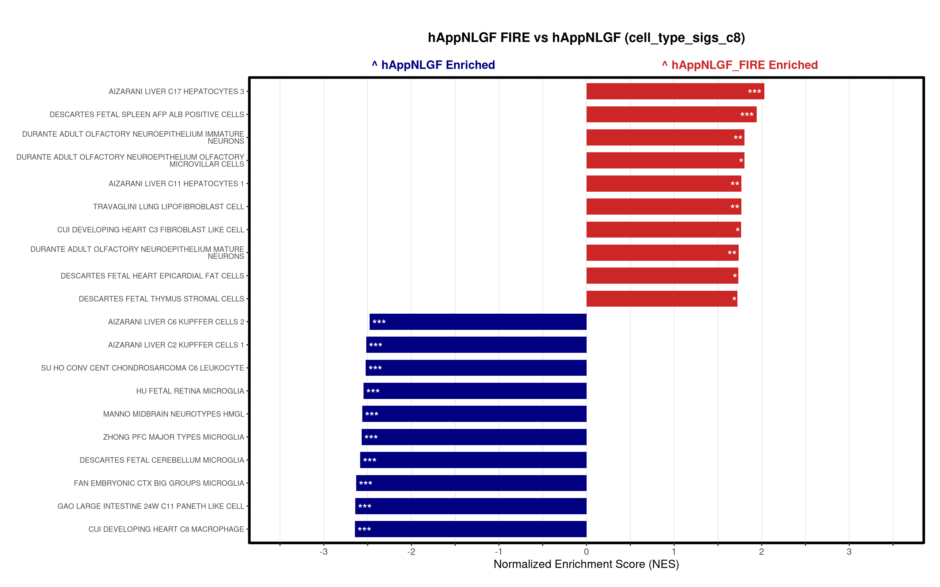
  "hAppNLGF_FIRE_vs_hAppNLGF"   = prep_msstats_ranks(res_df, protein_dictionary, "hAppNLGF_FIRE_vs_hAppNLGF"),
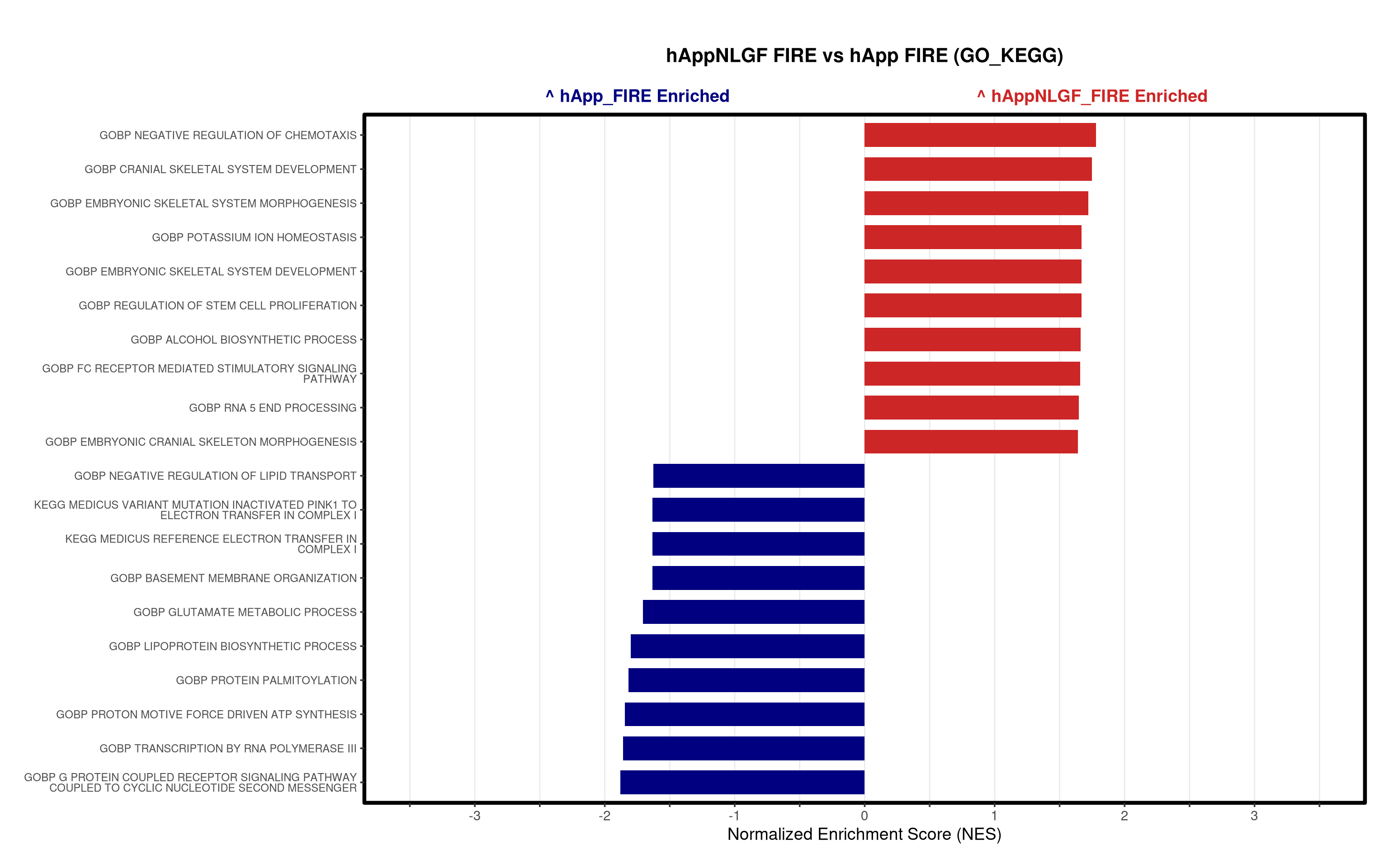
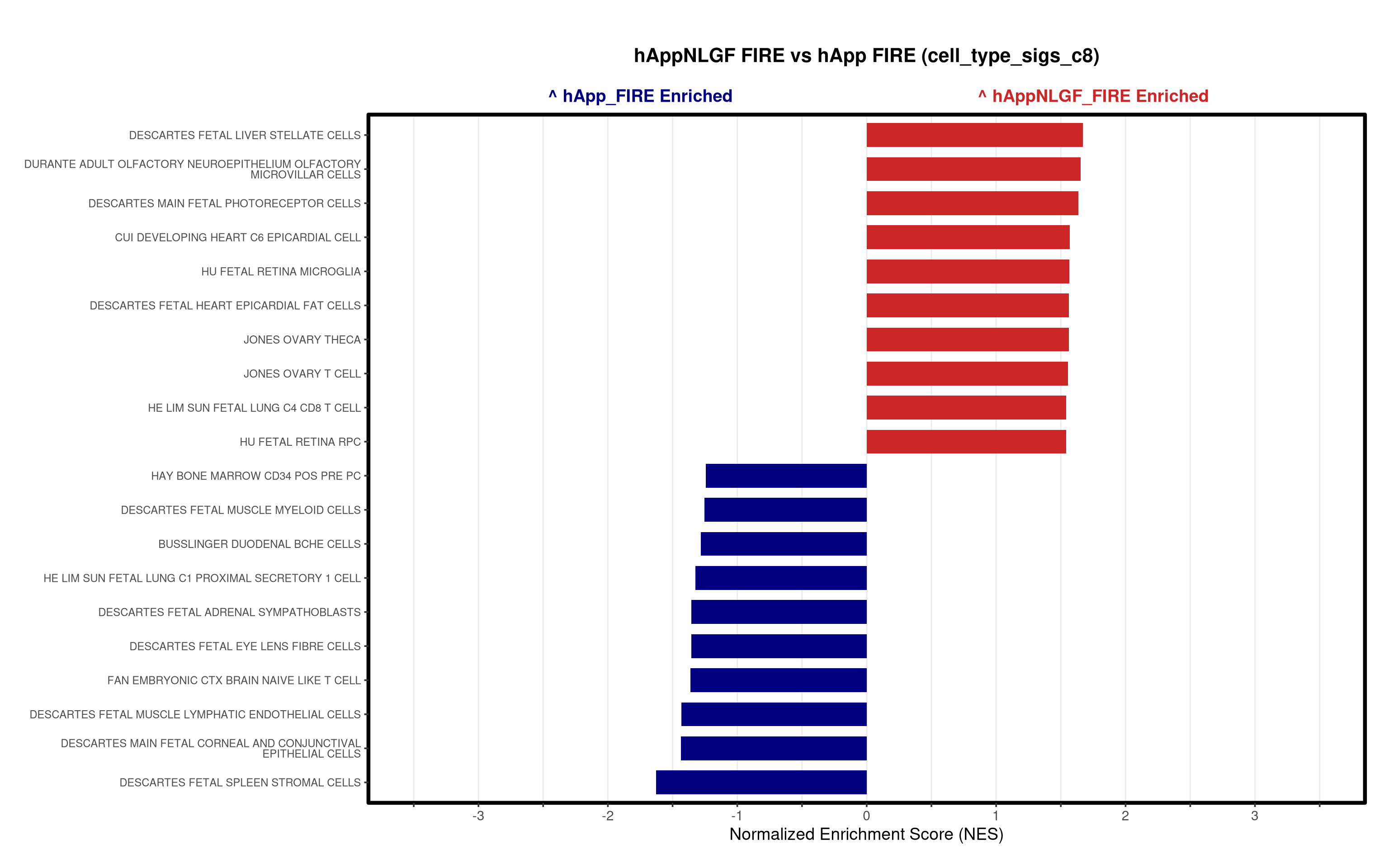
  "hAppNLGF_FIRE_vs_hApp_FIRE"  = prep_msstats_ranks(res_df, protein_dictionary, "hAppNLGF_FIRE_vs_hApp_FIRE")
)

Execute the GSEA function

Code

# ==============================================================================
# 3. EXECUTION LOOP
# ==============================================================================

purrr::walk2(names(gene_sets_master), gene_sets_master, function(gset_name, gset_pathways) {
  purrr::walk2(comparisons_master, names(comparisons_master), function(ranks, comp_name) {
    
    run_gsea_analysis(
      ranks            = ranks,
      comparison_name  = comp_name,
      geneset_name     = gset_name,     
      pathways         = gset_pathways, 
      base_objects_dir = objects_dir,   
      base_graphs_dir  = results_dir,    
      color_A          = GLOBAL_CONFIG$col_A,
      color_B          = GLOBAL_CONFIG$col_B
    )
    
    gc() # Memory cleanup
  })
})

Specific term plotting

Code

# ==============================================================================
# SPECIFIC TERM PLOTTING
# ==============================================================================

term_to_plot <- "GOBP_PLATELET_AGGREGATION"
# 1. Flatten master gene list
all_pathways_flat <- do.call(c, unname(gene_sets_master))

# Check if the term exists before looping - in case typo
if (!term_to_plot %in% names(all_pathways_flat)) {
  stop(glue("Could not find pathway '{term_to_plot}' in gene_sets_master."))
}

pathway_genes <- all_pathways_flat[[term_to_plot]]

# Create a specific output folder
specific_graphs_dir <- file.path(results_dir, "Specific_Pathway_Plots")
dir.create(specific_graphs_dir, showWarnings = FALSE, recursive = TRUE)

# Loop and Plot
purrr::walk2(comparisons_master, names(comparisons_master), function(ranks, comp_name) {
  
  message(glue("Plotting {term_to_plot} for {comp_name}..."))
  
  # Generate the GSEA enrichment plot
  gsea_plot <- plotEnrichment(pathway_genes, ranks) +
    labs(
      title = term_to_plot,
      subtitle = glue("Comparison: {comp_name}"),
      x = "Rank",
      y = "Enrichment Score"
    ) +
    theme_bw(base_size = 14) +
    theme(
      plot.title = element_text(face = "bold", hjust = 0.5),
      plot.subtitle = element_text(hjust = 0.5, color = "grey40"),
      panel.grid = element_blank()
    )
  print(gsea_plot)
  
  # Save
  ggsave(
    filename = file.path(specific_graphs_dir, glue("{term_to_plot}_{comp_name}.pdf")),
    plot = gsea_plot,
    width = 8, 
    height = 5
  )
})

Hypergeometric test: top 10 contrast genes vs top 10 leading-edge genes of a pathway

Tests whether the top 10 up-regulated proteins from a given MSstats contrast overlap the top 10 leading-edge genes of a chosen pathway more than expected by chance. Background = all genes present in that contrast’s rank vector.

Code

target_comparison <- "hAppNLGF_FIRE_vs_hAppNLGF"  # change to any of the four contrasts
target_pathway    <- term_to_plot                  # GOBP_LEUKOCYTE_MEDIATED_IMMUNITY by default

# Top 10 up-regulated genes from the chosen contrast
ranks_target <- comparisons_master[[target_comparison]]
top10_contrast <- ranks_target %>%
  sort(decreasing = TRUE) %>%
  head(10) %>%
  names()

# Top 10 leading-edge genes from the chosen pathway in that contrast
pathway_genes_upper <- toupper(all_pathways_flat[[target_pathway]])
set.seed(42)
fgsea_single <- fgsea(
  pathways    = list(sel = pathway_genes_upper),
  stats       = ranks_target,
  minSize     = 15,
  maxSize     = 3000,
  nPermSimple = 10000,
  BPPARAM     = BiocParallel::MulticoreParam(workers = 4, progressbar = FALSE)
)
leading_edge_genes <- fgsea_single$leadingEdge[[1]]
top10_pathway <- head(leading_edge_genes, 10)

# Background = all ranked genes in this contrast
background_genes <- names(ranks_target)
N <- length(background_genes)

overlap <- intersect(top10_contrast, top10_pathway)
k <- length(overlap)                              # observed overlap
m <- sum(top10_pathway %in% background_genes)     # pathway top10 present in background
n <- N - m                                        # genes NOT in pathway top10
q <- length(top10_contrast)                       # size of contrast top10

# phyper(k-1, ..., lower.tail = FALSE) gives P(X >= k)
p_val <- phyper(k - 1, m, n, q, lower.tail = FALSE)

cat(glue("=== Hypergeometric Test: {target_comparison} top10 vs {target_pathway} top10 ===\n"))

=== Hypergeometric Test: hAppNLGF_FIRE_vs_hAppNLGF top10 vs GOBP_PLATELET_AGGREGATION top10 ===

Code

cat("Background (total ranked proteins):", N, "\n")

Background (total ranked proteins): 8862

Code

cat("Pathway top 10 genes found in background:", m, "\n")

Pathway top 10 genes found in background: 10

Code

cat("Contrast top 10 proteins:", q, "\n")

Contrast top 10 proteins: 10

Code

cat("Observed overlap:", k, "\n")

Observed overlap: 0

Code

cat("Overlapping genes:", paste(overlap, collapse = ", "), "\n")

Overlapping genes:

Code

cat("P-value:", p_val, "\n\n")

P-value: 1

Code

overlap_df <- data.frame(
  Gene = background_genes,
  In_Pathway_Top10  = background_genes %in% top10_pathway,
  In_Contrast_Top10 = background_genes %in% top10_contrast
) %>%
  filter(In_Pathway_Top10 | In_Contrast_Top10) %>%
  mutate(Overlap = In_Pathway_Top10 & In_Contrast_Top10) %>%
  arrange(desc(Overlap))

print(overlap_df)

     Gene In_Pathway_Top10 In_Contrast_Top10 Overlap
1    IL34            FALSE              TRUE   FALSE
2     NNT            FALSE              TRUE   FALSE
3  CX3CL1            FALSE              TRUE   FALSE
4   MCPT4            FALSE              TRUE   FALSE
5    RTP1            FALSE              TRUE   FALSE
6     HYI            FALSE              TRUE   FALSE
7   S100Z            FALSE              TRUE   FALSE
8  TPSAB1            FALSE              TRUE   FALSE
9     OMP            FALSE              TRUE   FALSE
10 S100A5            FALSE              TRUE   FALSE
11 SLC6A4             TRUE             FALSE   FALSE
12   F11R             TRUE             FALSE   FALSE
13  ITGB3             TRUE             FALSE   FALSE
14    LYN             TRUE             FALSE   FALSE
15 ENTPD1             TRUE             FALSE   FALSE
16    SYK             TRUE             FALSE   FALSE
17   PLEK             TRUE             FALSE   FALSE
18  PTPN6             TRUE             FALSE   FALSE
19 FERMT3             TRUE             FALSE   FALSE
20 P2RY12             TRUE             FALSE   FALSE