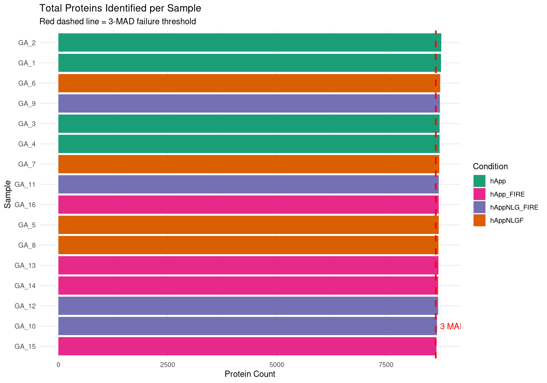
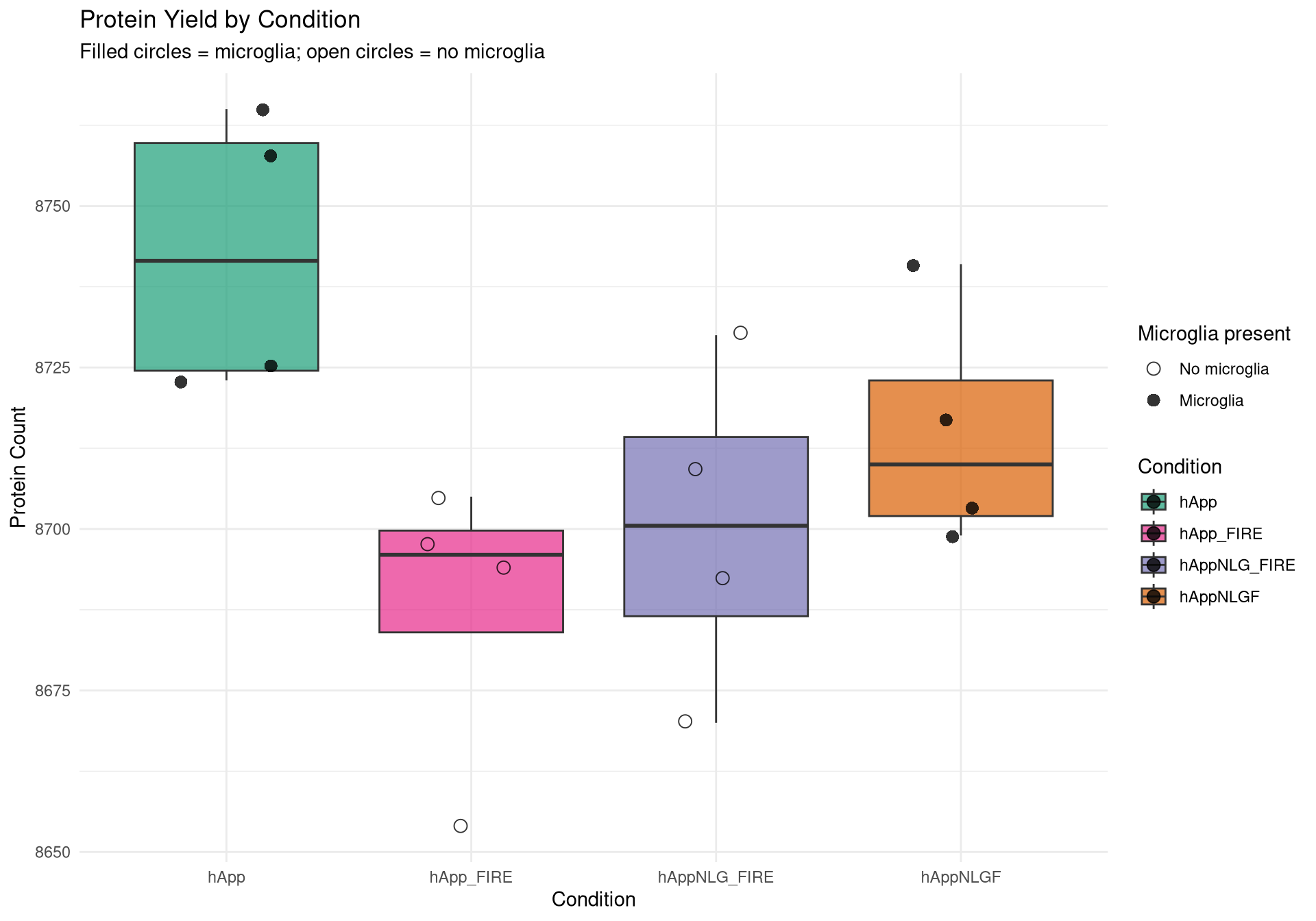
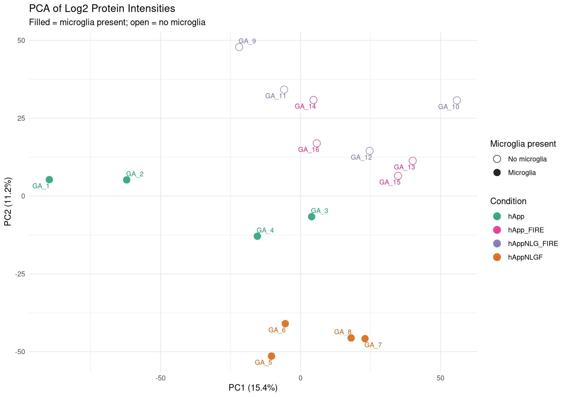
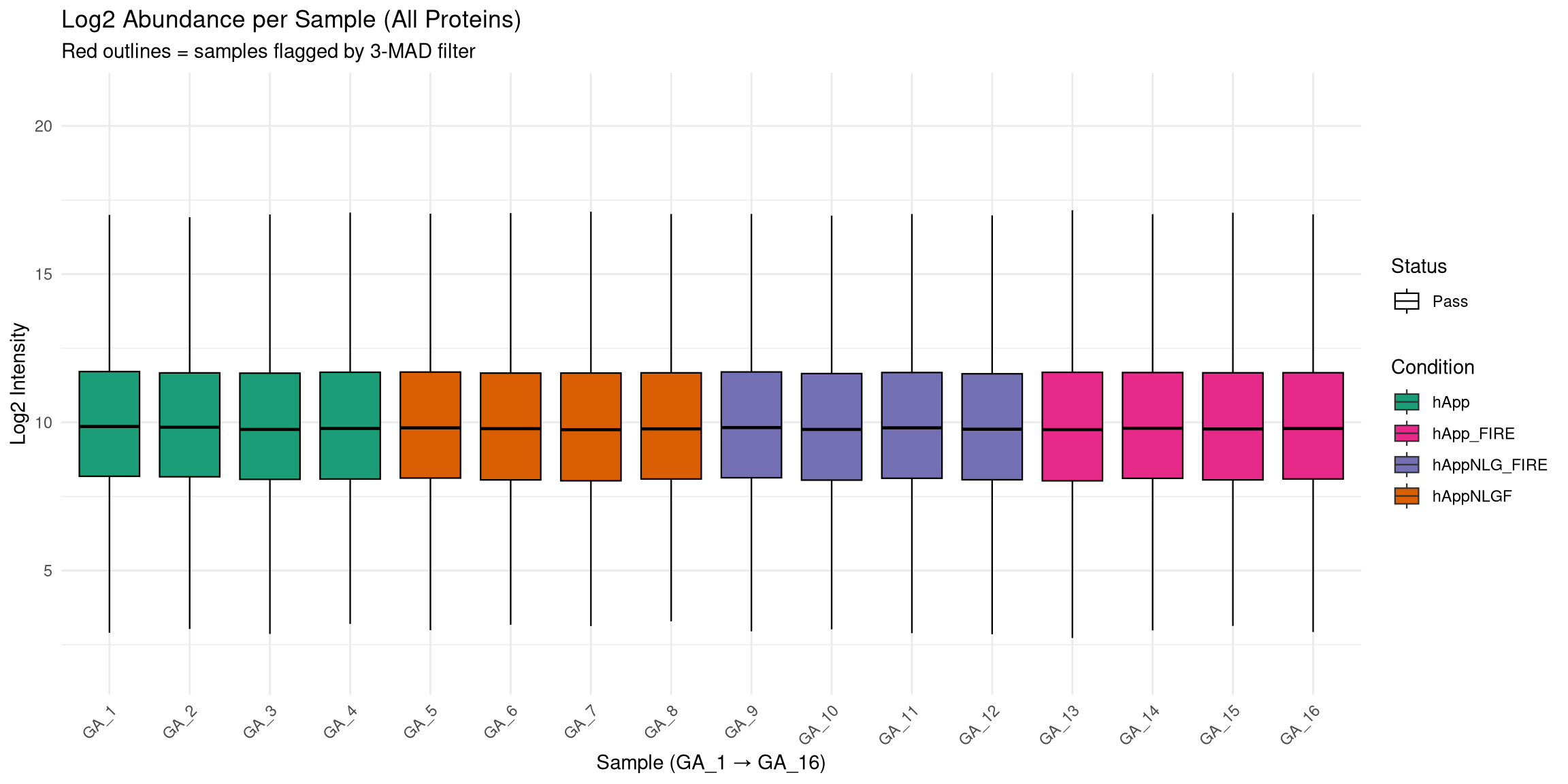
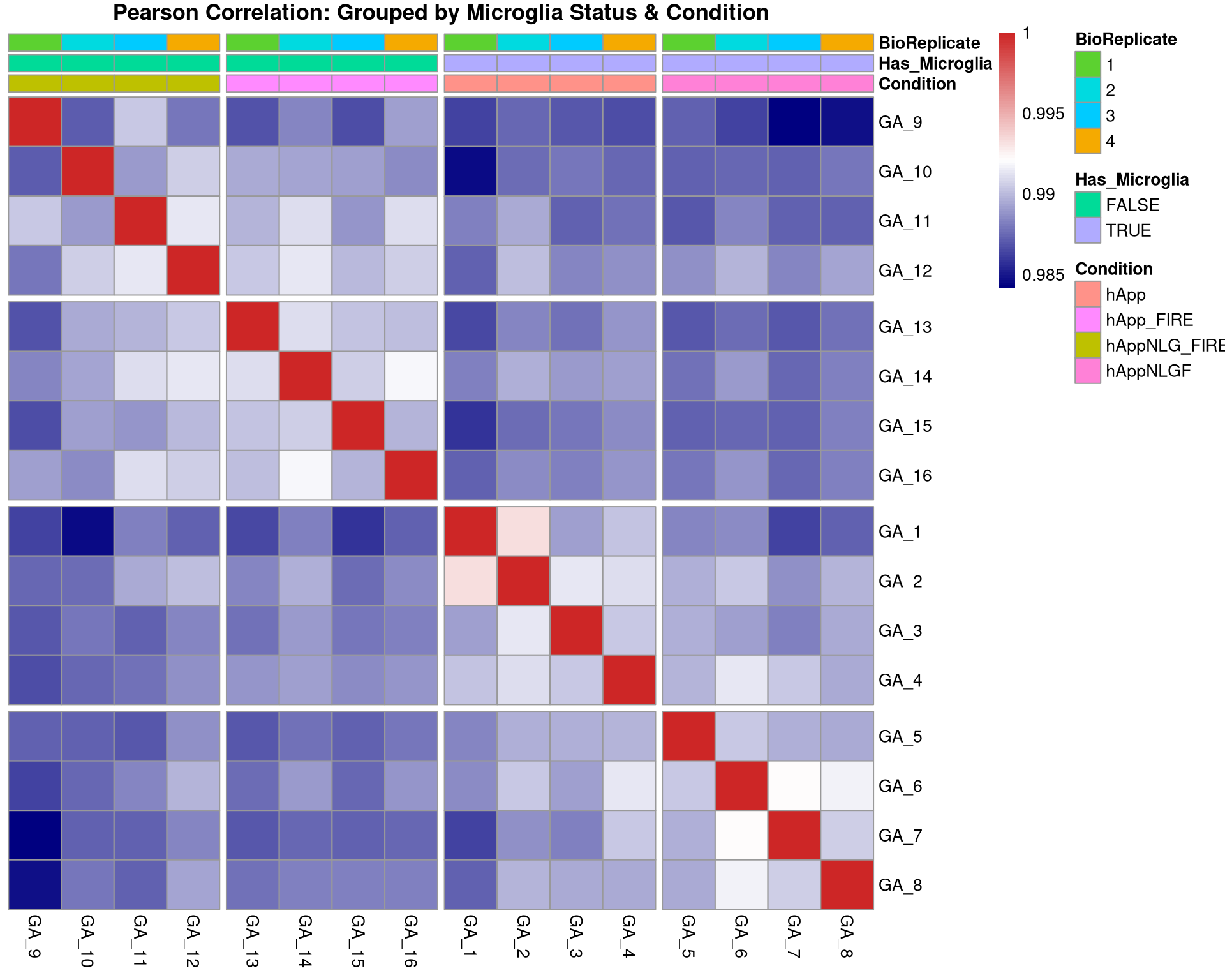
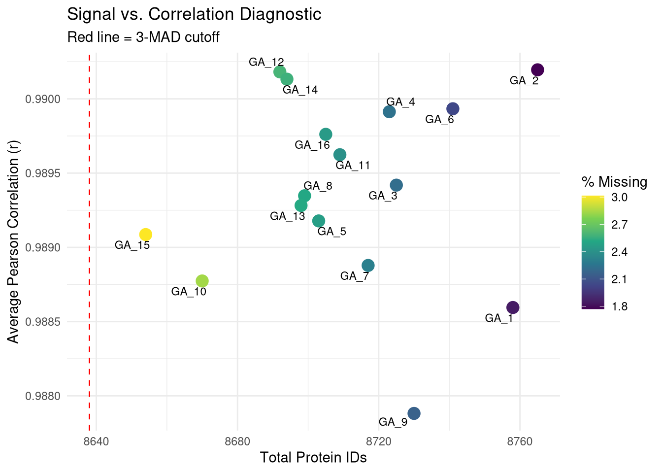
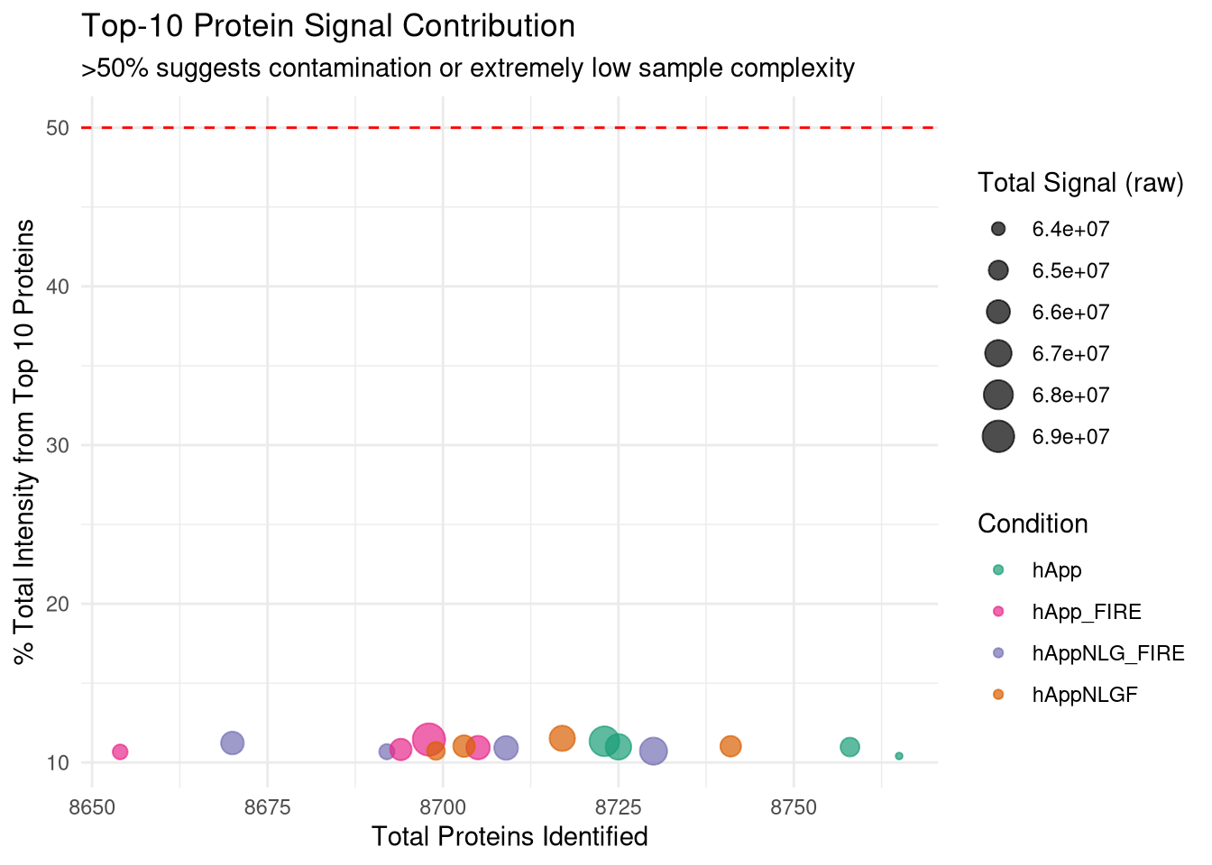
Initial QC & Data Cleaning — Proteome

Libraries

Set directories

Code

base_dir <- "/nemo/lab/destrooperb/home/shared/zanettc/giulia_proteomics/bulk_proteomics"
run_num  <- "run4"

results_dir <- file.path(base_dir, "results", run_num)
objects_dir <- file.path(base_dir, "data", "processed", run_num)
input_dir   <- file.path(base_dir, "input")

dir.create(results_dir, recursive = TRUE, showWarnings = FALSE)
dir.create(objects_dir, recursive = TRUE, showWarnings = FALSE)

Define study design

GA_1–4: hApp | GA_5–8: hAppNLGF | GA_9–12: hAppNLG_FIRE (no microglia) | GA_13–16: hApp_FIRE (no microglia)

Code

meta <- data.table(
  FileName      = paste0("GA_", 1:16),
  Condition     = rep(c("hApp", "hAppNLGF", "hAppNLG_FIRE", "hApp_FIRE"), each = 4),
  BioReplicate  = rep(1:4, times = 4),
  Has_Microglia = rep(c(TRUE, TRUE, FALSE, FALSE), each = 4)
)
meta

Read Spectronaut MSStats proteome report

Only the protein-level columns are selected to keep memory manageable on this 8.4 GB file. After deduplication the fragment-level rows collapse to one row per protein–sample pair.

Code

cat("Reading Spectronaut report (selecting protein-level columns only)...\n")

Reading Spectronaut report (selecting protein-level columns only)...

Code

#no PG.Genes
spec_raw <- fread(
  file.path(input_dir, "20260423_154110_PCF000612_GA_MSStats_Report-Proteome.csv")#,
  #select = c("R.FileName", "PG.ProteinGroups", "PG.ProteinAccessions", #"PG.Qvalue", "PG.Quantity")
)

cat("Fragment rows loaded:", nrow(spec_raw), "\n")

Fragment rows loaded: 24057952

Code

cat("Unique samples found:", uniqueN(spec_raw$R.FileName), "\n")

Unique samples found: 16

Code

cat("Samples present:", sort(unique(spec_raw$R.FileName)), "\n")

Samples present: GA_1 GA_10 GA_11 GA_12 GA_13 GA_14 GA_15 GA_16 GA_2 GA_3 GA_4 GA_5 GA_6 GA_7 GA_8 GA_9

Extract unique protein-level quantities per sample

PG.Quantity repeats for every fragment of a protein within a sample — deduplicate to one row per protein–sample pair.

Code

pg_long <- unique(spec_raw[, .(R.FileName, PG.ProteinGroups, PG.ProteinAccessions,
                                PG.Qvalue, PG.Quantity)])

cat("Unique protein-sample rows:", nrow(pg_long), "\n")

Unique protein-sample rows: 142768

Code

cat("Unique proteins:", uniqueN(pg_long$PG.ProteinGroups), "\n")

Unique proteins: 8923

Pivot to wide format (proteins × samples)

Code

quant_wide <- dcast(
  pg_long[, .(R.FileName, PG.ProteinGroups, PG.Quantity)],
  PG.ProteinGroups ~ R.FileName,
  value.var = "PG.Quantity"
)

sample_cols <- paste0("GA_", 1:16)

# Sanity-check that all expected samples are present
missing_samples <- setdiff(sample_cols, colnames(quant_wide))
if (length(missing_samples) > 0) {
  warning("These samples are missing from the data: ", paste(missing_samples, collapse = ", "))
} else {
  cat("All 16 samples found in data.\n")
}

All 16 samples found in data.

Code

# Extract quantitative matrix in numeric order (GA_1 … GA_16)
quant_data <- quant_wide[, ..sample_cols]

# Convert Spectronaut NaN to R NA throughout
quant_matrix <- as.matrix(quant_data)
quant_matrix[is.nan(quant_matrix)] <- NA

cat("Proteins in matrix:", nrow(quant_matrix), "\n")

Proteins in matrix: 8923

Code

cat("Samples in matrix: ", ncol(quant_matrix), "\n")

Samples in matrix:  16

Calculate protein ID counts per sample

A protein is “identified” if it has a finite, positive PG.Quantity.

Code

protein_counts <- colSums(!is.na(quant_matrix) & quant_matrix > 0)

qc_counts <- data.table(FileName = names(protein_counts), Protein_Count = protein_counts)
qc_data   <- merge(qc_counts, meta, by = "FileName", all.x = TRUE)

summary(qc_data$Protein_Count)

   Min. 1st Qu.  Median    Mean 3rd Qu.    Max. 
   8654    8697    8707    8711    8726    8765

Code

qc_data

MAD outlier detection

Flags samples with protein counts more than 3 MADs below the median.

Code

med_count  <- median(qc_data$Protein_Count, na.rm = TRUE)
mad_count  <- mad(qc_data$Protein_Count, na.rm = TRUE)
mad_cutoff <- med_count - (3 * mad_count)

cat("Median Protein Count:", round(med_count), "\n")

Median Protein Count: 8707

Code

cat("MAD:                 ", round(mad_count), "\n")

MAD:                  23

Code

cat("3-MAD cutoff:        ", round(mad_cutoff), "\n")

3-MAD cutoff:         8638

Code

failed_runs <- qc_data[Protein_Count < mad_cutoff, FileName]

if (length(failed_runs) > 0) {
  cat("\nWARNING:", length(failed_runs), "failed run(s) to drop:\n")
  print(failed_runs)
} else {
  cat("\nNo runs fell below the 3-MAD threshold.\n")
}


No runs fell below the 3-MAD threshold.

Generate PDF QC report

Code

condition_colours <- c(
  "hApp"         = "#1b9e77",
  "hAppNLGF"     = "#d95f02",
  "hAppNLG_FIRE" = "#7570b3",
  "hApp_FIRE"    = "#e7298a"
)

# ── Plot 1: Protein Count per Sample with MAD cutoff ───────────────────────
p1 <- ggplot(qc_data,
             aes(x = reorder(FileName, Protein_Count), y = Protein_Count, fill = Condition)) +
  geom_bar(stat = "identity") +
  geom_hline(yintercept = mad_cutoff, color = "red", linetype = "dashed", linewidth = 1) +
  annotate("text", x = 2, y = mad_cutoff + 100,
           label = "3 MAD Cutoff", color = "red", hjust = 0) +
  scale_fill_manual(values = condition_colours) +
  coord_flip() +
  theme_minimal() +
  labs(title = "Total Proteins Identified per Sample",
       subtitle = "Red dashed line = 3-MAD failure threshold",
       x = "Sample", y = "Protein Count") +
  theme(axis.text.y = element_text(size = 9))

# ── Plot 2: Protein Yield by Condition ─────────────────────────────────────
p2 <- ggplot(qc_data, aes(x = Condition, y = Protein_Count, fill = Condition)) +
  geom_boxplot(outlier.shape = NA, alpha = 0.7) +
  geom_point(aes(shape = Has_Microglia),
             position = position_jitter(width = 0.2), alpha = 0.8, size = 3) +
  scale_fill_manual(values = condition_colours) +
  scale_shape_manual(values = c("TRUE" = 16, "FALSE" = 1),
                     labels = c("TRUE" = "Microglia", "FALSE" = "No microglia")) +
  theme_minimal() +
  labs(title = "Protein Yield by Condition",
       subtitle = "Filled circles = microglia; open circles = no microglia",
       x = "Condition", y = "Protein Count",
       shape = "Microglia present")

# ── PCA ─────────────────────────────────────────────────────────────────────
cat("Preparing PCA...\n")

Preparing PCA...

Code

pca_mat_log   <- log2(quant_matrix + 1)
pca_mat_log_t <- t(pca_mat_log)

noise_floor <- min(pca_mat_log_t[pca_mat_log_t > 0], na.rm = TRUE) / 2
pca_mat_log_t[is.na(pca_mat_log_t) | pca_mat_log_t == 0] <- noise_floor

valid_cols    <- apply(pca_mat_log_t, 2, var) > 0
pca_mat_log_t <- pca_mat_log_t[, valid_cols]
cat("Proteins retained for PCA (non-zero variance):", sum(valid_cols), "\n")

Proteins retained for PCA (non-zero variance): 8792

Code

pca_res  <- prcomp(pca_mat_log_t, center = TRUE, scale. = TRUE)
var_expl <- round(100 * pca_res$sdev^2 / sum(pca_res$sdev^2), 1)

pca_df <- as.data.frame(pca_res$x)
pca_df$FileName <- rownames(pca_df)
pca_df <- merge(pca_df, meta, by = "FileName", all.x = TRUE)

# ── Plot 3: PCA by Condition ────────────────────────────────────────────────
p3 <- ggplot(pca_df, aes(x = PC1, y = PC2, color = Condition, shape = Has_Microglia)) +
  geom_point(size = 4, alpha = 0.85) +
  ggrepel::geom_text_repel(aes(label = FileName), size = 3, max.overlaps = 20) +
  scale_color_manual(values = condition_colours) +
  scale_shape_manual(values = c("TRUE" = 16, "FALSE" = 1),
                     labels = c("TRUE" = "Microglia", "FALSE" = "No microglia")) +
  theme_minimal() +
  labs(title = "PCA of Log2 Protein Intensities",
       subtitle = "Filled = microglia present; open = no microglia",
       x = paste0("PC1 (", var_expl[1], "%)"),
       y = paste0("PC2 (", var_expl[2], "%)"),
       shape = "Microglia present")

# ── Save PDF ────────────────────────────────────────────────────────────────
pdf_path <- file.path(results_dir, "Initial_QC_Report.pdf")
cat("Saving PDF:", pdf_path, "\n")

Saving PDF: /nemo/lab/destrooperb/home/shared/zanettc/giulia_proteomics/bulk_proteomics/results/run4/Initial_QC_Report.pdf

Code

pdf(pdf_path, width = 10, height = 7)
print(p1); print(p2); print(p3)
dev.off()

png 
  2

Code

print(p1); print(p2); print(p3)

Abundance distributions

Log2 intensity boxplots per sample, ordered numerically. Red outlines flag MAD failures.

Code

quant_log_plot <- log2(quant_matrix + 1)
quant_log_plot[quant_log_plot == 0] <- NA

abund_long <- as.data.frame(quant_log_plot) %>%
  mutate(Protein = row_number()) %>%
  pivot_longer(-Protein, names_to = "FileName", values_to = "Log2_Intensity") %>%
  drop_na() %>%
  left_join(as.data.frame(qc_data), by = "FileName") %>%
  mutate(
    Status      = ifelse(FileName %in% failed_runs, "Failed (Outlier)", "Pass"),
    Sample_Num  = as.integer(str_extract(FileName, "[0-9]+"))
  )

p_abund <- ggplot(abund_long, aes(x = reorder(FileName, Sample_Num),
                                   y = Log2_Intensity, fill = Condition)) +
  geom_boxplot(aes(color = Status), outlier.shape = NA, lwd = 0.4) +
  scale_fill_manual(values = condition_colours) +
  scale_color_manual(values = c("Pass" = "black", "Failed (Outlier)" = "red")) +
  theme_minimal() +
  labs(title = "Log2 Abundance per Sample (All Proteins)",
       subtitle = "Red outlines = samples flagged by 3-MAD filter",
       x = "Sample (GA_1 → GA_16)", y = "Log2 Intensity") +
  theme(axis.text.x = element_text(angle = 45, hjust = 1))

print(p_abund)

Correlation heatmap

Samples grouped by microglia status then condition to make the biological structure visible.

Code

quant_mat_cor <- log2(quant_matrix + 1)
quant_mat_cor[quant_mat_cor == 0] <- NA

cor_mat <- cor(quant_mat_cor, use = "pairwise.complete.obs")

meta_sorted <- meta %>%
  arrange(Has_Microglia, Condition, BioReplicate) %>%
  as.data.frame()

sorted_runs    <- meta_sorted$FileName
cor_mat_sorted <- cor_mat[sorted_runs, sorted_runs]

anno_df <- meta_sorted %>%
  select(FileName, Condition, Has_Microglia, BioReplicate) %>%
  mutate(Has_Microglia = as.factor(Has_Microglia),
         BioReplicate  = as.factor(BioReplicate)) %>%
  as.data.frame()
rownames(anno_df) <- anno_df$FileName
anno_df$FileName  <- NULL

pheatmap(cor_mat_sorted,
         main           = "Pearson Correlation: Grouped by Microglia Status & Condition",
         annotation_col = anno_df,
         cluster_rows   = FALSE,
         cluster_cols   = FALSE,
         show_rownames  = TRUE,
         show_colnames  = TRUE,
         color          = colorRampPalette(c("navy", "white", "firebrick3"))(100),
         gaps_col       = which(diff(as.numeric(as.factor(meta_sorted$Condition))) != 0),
         gaps_row       = which(diff(as.numeric(as.factor(meta_sorted$Condition))) != 0))

Average-correlation diagnostic

Identifies the sample with the lowest mean correlation to the rest of the cohort.

Code

qc_diagnostics <- data.table(
  FileName        = colnames(quant_mat_cor),
  Protein_Count   = protein_counts[colnames(quant_mat_cor)],
  NA_Percent      = colMeans(is.na(quant_mat_cor)) * 100,
  Avg_Correlation = rowMeans(cor_mat, na.rm = TRUE)
)

outlier_id <- qc_diagnostics[which.min(Avg_Correlation), FileName]

cat("--- Diagnostic for lowest-correlation sample ---\n")

--- Diagnostic for lowest-correlation sample ---

Code

print(qc_diagnostics[FileName == outlier_id])

   FileName Protein_Count NA_Percent Avg_Correlation
     <char>         <num>      <num>           <num>
1:     GA_9          8730    2.16295       0.9878816

Code

p_diag <- ggplot(qc_diagnostics, aes(x = Protein_Count, y = Avg_Correlation)) +
  geom_point(aes(color = NA_Percent), size = 4) +
  geom_vline(xintercept = mad_cutoff, linetype = "dashed", color = "red") +
  ggrepel::geom_text_repel(aes(label = FileName), size = 3, max.overlaps = 20) +
  scale_color_viridis_c(name = "% Missing") +
  theme_minimal() +
  labs(title = "Signal vs. Correlation Diagnostic",
       subtitle = "Red line = 3-MAD cutoff",
       x = "Total Protein IDs", y = "Average Pearson Correlation (r)")

print(p_diag)

Contaminant check: top-10 protein signal contribution

High top-10% (>50%) suggests a very low-complexity sample or dominant contaminant proteins (e.g. keratins, actin).

Code

calc_top_n_pct <- function(column, n = 10) {
  sorted_vals <- sort(column, decreasing = TRUE, na.last = TRUE)
  (sum(sorted_vals[1:n], na.rm = TRUE) / sum(column, na.rm = TRUE)) * 100
}

top10_metrics <- apply(quant_matrix, 2, calc_top_n_pct, n = 10)
qc_data[, Top10_Percent   := top10_metrics[FileName]]
qc_data[, Total_Intensity := colSums(quant_matrix, na.rm = TRUE)[FileName]]

contaminant_suspects <- qc_data[Top10_Percent > 50,
                                 .(FileName, Condition, Protein_Count, Top10_Percent)]
cat("Samples where top 10 proteins account for >50% of signal:\n")

Samples where top 10 proteins account for >50% of signal:

Code

print(contaminant_suspects)

Key: <FileName>
Empty data.table (0 rows and 4 cols): FileName,Condition,Protein_Count,Top10_Percent

Code

p_top10 <- ggplot(qc_data, aes(x = Protein_Count, y = Top10_Percent)) +
  geom_point(aes(color = Condition, size = Total_Intensity), alpha = 0.7) +
  geom_hline(yintercept = 50, linetype = "dashed", color = "red") +
  ggrepel::geom_text_repel(
    aes(label = ifelse(Top10_Percent > 50, FileName, "")),
    size = 3, max.overlaps = 10
  ) +
  scale_color_manual(values = condition_colours) +
  theme_minimal() +
  labs(title = "Top-10 Protein Signal Contribution",
       subtitle = ">50% suggests contamination or extremely low sample complexity",
       x = "Total Proteins Identified",
       y = "% Total Intensity from Top 10 Proteins",
       size = "Total Signal (raw)")

print(p_top10)

Identify top contributing proteins in suspect samples

Code

if (nrow(contaminant_suspects) > 0) {
  suspect_cols <- contaminant_suspects$FileName
  top_ids <- apply(quant_matrix[, suspect_cols, drop = FALSE], 2, function(x) {
    quant_wide$PG.ProteinGroups[which.max(x)]
  })
  cat("Top protein per suspect sample:\n")
  print(top_ids)
} else {
  cat("No suspect samples to investigate.\n")
}

No suspect samples to investigate.

Filter out failed samples

Code

valid_runs <- meta$FileName
final_runs <- setdiff(valid_runs, failed_runs)

cat("Original samples:        ", length(valid_runs), "\n")

Original samples:         16

Code

cat("Samples dropped (3-MAD): ", length(failed_runs), "\n")

Samples dropped (3-MAD):  0

Code

cat("Clean samples remaining: ", length(final_runs), "\n")

Clean samples remaining:  16

Code

if (length(failed_runs) > 0) print(failed_runs)

Save objects

Code

# Clean wide protein matrix (proteins × passing samples)
clean_quant_wide <- cbind(
  quant_wide[, .(PG.ProteinGroups)],
  quant_wide[, ..final_runs]
)

# Clean metadata
clean_meta <- qc_data[FileName %in% final_runs]

# Dropped sample log
dropped_log <- qc_data[FileName %in% failed_runs,
                        .(FileName, Condition, Has_Microglia, Protein_Count)]
dropped_log[, Reason := "Sub 3-MAD Protein Count"]


fwrite(spec_raw, file.path(objects_dir, "clean_spec_raw.csv"))
fwrite(clean_meta,       file.path(objects_dir, "clean_metadata.csv"))
fwrite(clean_quant_wide, file.path(objects_dir, "clean_quant_wide.csv"))
fwrite(dropped_log,      file.path(objects_dir, "dropped_samples_log.csv"))

cat("Objects saved to:", objects_dir, "\n")

Objects saved to: /nemo/lab/destrooperb/home/shared/zanettc/giulia_proteomics/bulk_proteomics/data/processed/run4