Code
library(data.table)
library(MSstats)
library(qs2)
library(dplyr)
library(ggplot2)
library(ggrepel)
library(tidyverse)
library(readr)library(data.table)
library(MSstats)
library(qs2)
library(dplyr)
library(ggplot2)
library(ggrepel)
library(tidyverse)
library(readr)base_dir <- "/nemo/lab/destrooperb/home/shared/zanettc/giulia_proteomics/bulk_proteomics"
run_num <- "run4"
results_dir <- file.path(base_dir, "results", run_num)
objects_dir <- file.path(base_dir, "data", "processed", run_num)
input_dir <- file.path(base_dir, "input")
dir.create(results_dir, recursive = TRUE, showWarnings = FALSE)
dir.create(objects_dir, recursive = TRUE, showWarnings = FALSE)All 16 samples passed QC. R.Condition = “Not Defined” in the raw file because the study design was not configured inside Spectronaut — we define it here from the known design.
msstats_annotation <- data.table(
  Run          = paste0("GA_", 1:16),
  Condition    = rep(c("hApp", "hAppNLGF", "hAppNLGF_FIRE", "hApp_FIRE"), each = 4),
  BioReplicate = 1:16
)
msstats_annotationfwrite(msstats_annotation, file.path(objects_dir, "msstats_annotation.csv"))Only the columns required by MSstats are read — this keeps memory manageable on the 8.4 GB file.
msstats_cols <- c(
  "R.Condition", "R.FileName", "R.Replicate",
  "PG.ProteinGroups", "PG.ProteinAccessions",
  "PEP.StrippedSequence",
  "EG.ModifiedSequence", "EG.PrecursorId", "EG.Qvalue",
  "FG.Charge", "FG.Id",
  "F.FrgIon", "F.Charge", "F.FrgLossType", "F.FrgNum", "F.FrgType",
  "F.NormalizedPeakArea", "F.PeakArea", "F.ExcludedFromQuantification"
)

cat("Reading Spectronaut MSstats report...\n")
Reading Spectronaut MSstats report...raw_spectronaut <- fread(
file.path(input_dir, "20260423_154110_PCF000612_GA_MSStats_Report-Proteome.csv"),
select = msstats_cols
)
cat("Rows loaded:", nrow(raw_spectronaut), "\n")Rows loaded: 24057952 qs_save(raw_spectronaut, file.path(objects_dir, "msstats_report.qs2"))#raw_spectronaut <- qs_read(file.path(objects_dir, "msstats_report.qs2"))SpectronauttoMSstatsFormat uses R.Condition internally before merging with the annotation. We replace “Not Defined” with the correct values from the annotation to avoid any issues.
raw_spectronaut[msstats_annotation,
                on = c("R.FileName" = "Run"),
                `:=`(R.Condition = i.Condition,
                     R.Replicate = i.BioReplicate)]

cat("Condition distribution after fix:\n")
Condition distribution after fix:print(raw_spectronaut[, .N, by = .(R.Condition, R.FileName)][order(R.Condition, R.FileName)]) R.Condition R.FileName N
<char> <char> <int>
1: hApp GA_1 1503622
2: hApp GA_2 1503622
3: hApp GA_3 1503622
4: hApp GA_4 1503622
5: hAppNLGF GA_5 1503622
6: hAppNLGF GA_6 1503622
7: hAppNLGF GA_7 1503622
8: hAppNLGF GA_8 1503622
9: hAppNLGF_FIRE GA_10 1503622
10: hAppNLGF_FIRE GA_11 1503622
11: hAppNLGF_FIRE GA_12 1503622
12: hAppNLGF_FIRE GA_9 1503622
13: hApp_FIRE GA_13 1503622
14: hApp_FIRE GA_14 1503622
15: hApp_FIRE GA_15 1503622
16: hApp_FIRE GA_16 1503622Confirms that hApp and hAppNLGF conditions have detectable Aβ signal. In microglia, signal reflects phagocytosed / secreted Aβ rather than endogenous APP expression.
arctic_peptide <- "LVFFAGDVGSNK"
normal_peptide <- "LVFFAEDVGSNK"
peptide_both <- "DAEFRHDSGYEVHHQK"

target_peptide <- "LVFFAEDVGSNK"  # Conserved Aβ tryptic peptide (mouse and human APP)


ab_check <- raw_spectronaut %>%
  filter(PEP.StrippedSequence == target_peptide) %>%
  group_by(R.FileName, R.Condition) %>%
  summarise(Total_Intensity = sum(F.PeakArea, na.rm = TRUE), .groups = "drop") %>%
  mutate(Log2_Intensity = log2(Total_Intensity + 1)) %>%
  # Extract numeric sample ID for proper sorting
  mutate(Sample_Num = as.numeric(gsub("GA_", "", R.FileName))) %>%
  arrange(R.Condition, Sample_Num) %>%
  mutate(R.FileName = factor(R.FileName, levels = unique(R.FileName)))

if (nrow(ab_check) == 0) {
  cat("Aβ peptide (", target_peptide, ") not detected in any sample.\n")
} else {
  cat("Aβ peptide detected in", nrow(ab_check), "sample(s):\n")
  print(ab_check)
}
Aβ peptide detected in 16 sample(s):
# A tibble: 16 × 5
R.FileName R.Condition Total_Intensity Log2_Intensity Sample_Num
<fct> <chr> <dbl> <dbl> <dbl>
1 GA_1 hApp 3870. 11.9 1
2 GA_2 hApp 5470. 12.4 2
3 GA_3 hApp 2421. 11.2 3
4 GA_4 hApp 2905. 11.5 4
5 GA_5 hAppNLGF 25.4 4.72 5
6 GA_6 hAppNLGF 93.3 6.56 6
7 GA_7 hAppNLGF 25.3 4.72 7
8 GA_8 hAppNLGF 12.4 3.75 8
9 GA_9 hAppNLGF_FIRE 72.5 6.20 9
10 GA_10 hAppNLGF_FIRE 16.4 4.12 10
11 GA_11 hAppNLGF_FIRE 8.20 3.20 11
12 GA_12 hAppNLGF_FIRE 99.1 6.64 12
13 GA_13 hApp_FIRE 3174. 11.6 13
14 GA_14 hApp_FIRE 2566. 11.3 14
15 GA_15 hApp_FIRE 2386. 11.2 15
16 GA_16 hApp_FIRE 3082. 11.6 16p_ab <- ggplot(ab_check, aes(x = R.FileName, y = Log2_Intensity, fill = R.Condition)) +
geom_bar(stat = "identity") +
scale_fill_manual(values = c(
"hApp" = "#1b9e77", "hAppNLGF" = "#d95f02",
"hAppNLGF_FIRE" = "#7570b3", "hApp_FIRE" = "#e7298a"
)) +
theme_minimal() +
theme(axis.text.x = element_text(angle = 45, hjust = 1)) +
labs(title = "Aβ Tryptic Peptide Signal per Sample",
subtitle = paste0("Peptide: ", target_peptide),
x = "Sample", y = "Log2 Intensity")
ggsave(file.path(results_dir, "AB_Peptide_Verification.pdf"), p_ab, width = 10, height = 6)
print(p_ab)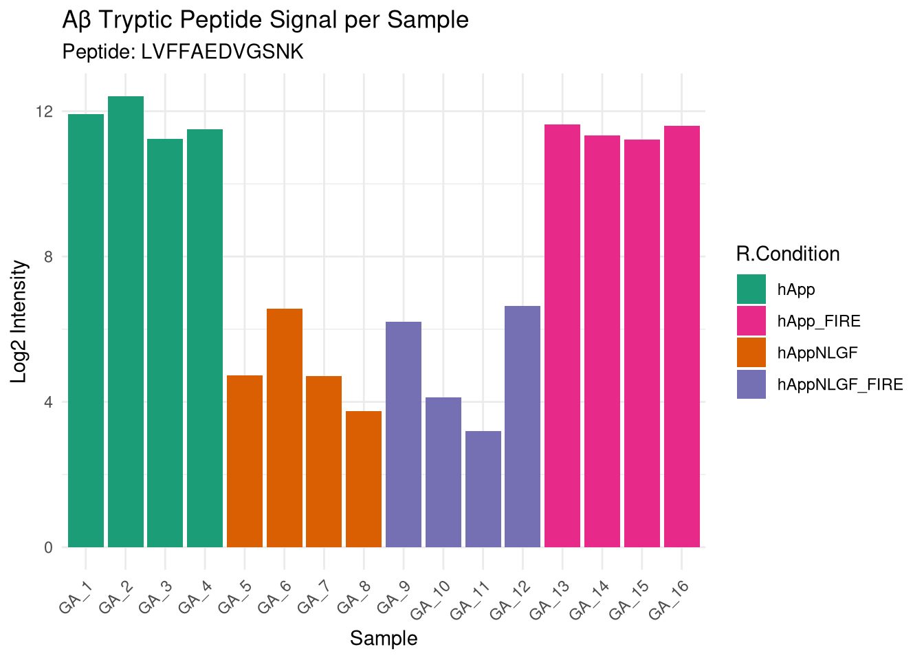
Feature-level filtering: Qvalue < 0.01, remove features with too few measurements.
msstats_input <- suppressWarnings(SpectronauttoMSstatsFormat(
  raw_spectronaut,
  annotation                  = msstats_annotation,
  filter_with_Qvalue          = TRUE,
  qvalue_cutoff               = 0.01,
  fewMeasurements             = "remove",
  removeProtein_with1Feature  = FALSE
))
INFO [2026-04-29 22:21:08] ** Raw data from Spectronaut imported successfully.
INFO [2026-04-29 22:21:14] ** Raw data from Spectronaut cleaned successfully.
INFO [2026-04-29 22:21:14] ** Using provided annotation.
INFO [2026-04-29 22:21:14] ** Run labels were standardized to remove symbols such as '.' or '%'.
INFO [2026-04-29 22:21:14] ** The following options are used:
- Features will be defined by the columns: PeptideSequence, PrecursorCharge, FragmentIon, ProductCharge
- Shared peptides will be removed.
- Proteins with single feature will not be removed.
- Features with less than 3 measurements across runs will be removed.
INFO [2026-04-29 22:21:20] ** Intensities with values of FExcludedFromQuantification equal to TRUE are replaced with NA
WARN [2026-04-29 22:21:23] ** PGQvalue not found in input columns.
INFO [2026-04-29 22:21:24] ** Intensities with values not smaller than 0.01 in EGQvalue are replaced with NA
INFO [2026-04-29 22:21:30] ** Features with all missing measurements across runs are removed.
INFO [2026-04-29 22:21:36] ** Shared peptides are removed.
INFO [2026-04-29 22:22:56] ** Multiple measurements in a feature and a run are summarized by summaryforMultipleRows: max
INFO [2026-04-29 22:23:00] ** Features with one or two measurements across runs are removed.
INFO [2026-04-29 22:23:02] ** Run annotation merged with quantification data.
INFO [2026-04-29 22:23:16] ** Features with one or two measurements across runs are removed.
INFO [2026-04-29 22:23:16] ** Fractionation handled.
INFO [2026-04-29 22:23:52] ** Updated quantification data to make balanced design. Missing values are marked by NA
INFO [2026-04-29 22:23:55] ** Finished preprocessing. The dataset is ready to be processed by the dataProcess function.cat("MSstats input rows:", nrow(msstats_input), "\n")MSstats input rows: 11946400 cat("Unique proteins: ", uniqueN(msstats_input$ProteinName), "\n")Unique proteins: 8918 qs_save(msstats_input, file.path(objects_dir, "msstats_input.qs2"))Keeps features observed in ≥50% of runs within at least one condition. This removes near-absent features that destabilise the linear model. This is the same as saying proteins must be present in at least 2 samples out of 3 for at least one condition.
# Manual resume only — not evaluated during render. msstats_input is already
# in memory from the chunk above; this line lets you skip rebuilding it on a re-run.
msstats_input <- qs_read(file.path(objects_dir, "msstats_input.qs2"))msstats_input_filt <- as.data.frame(msstats_input) %>%
group_by(ProteinName, PeptideSequence, PrecursorCharge, FragmentIon, ProductCharge, Condition) %>%
summarise(
n_obs = sum(!is.na(Intensity) & Intensity > 0),
n_total = n(),
prop = n_obs / n_total,
.groups = "drop"
) %>%
group_by(ProteinName, PeptideSequence, PrecursorCharge, FragmentIon, ProductCharge) %>%
filter(any(prop >= 0.5)) %>%
ungroup() %>%
inner_join(
as.data.frame(msstats_input),
by = c("ProteinName", "PeptideSequence", "PrecursorCharge",
"FragmentIon", "ProductCharge", "Condition")
)
message("Rows before completeness filter: ", nrow(msstats_input))
message("Rows after completeness filter: ", nrow(msstats_input_filt))
message("Proteins retained: ", uniqueN(msstats_input_filt$ProteinName))
table(
Value_Type = case_when(
is.na(msstats_input$Intensity) ~ "True NAs",
msstats_input$Intensity == 0 ~ "Exact Zeros (Filtered by Q-value)",
msstats_input$Intensity > 0 ~ "Valid Measurements"
)
)Value_Type
True NAs Valid Measurements
1736082 10210318 The MSstats report contains only UniProt accessions in ProteinName — no gene symbols. To filter keratins, build a lookup from UniProt or biomaRt and enable the block below.
## Keratin protein filter

protein_dict <- read_csv(file.path(base_dir, "data", "processed", "run1", "protein_dictionary.csv"))

# Pull all UniProt accessions annotated as keratin (Krt* gene symbol).
# The Protein column can be a semicolon-separated group, so split before matching.
keratin_ids <- protein_dict %>%
  filter(str_detect(Gene, "^Krt") & !str_detect(Gene, "^Krtcap")) %>%  # drop Krtcap2 (not a keratin contaminant)
  pull(Protein) %>%
  str_split(";") %>%
  unlist() %>%
  unique()

message("Keratin accessions to filter: ", length(keratin_ids))

# Match against ProteinName by splitting protein groups the same way,
# so a group is dropped if ANY member is a keratin.
msstats_input_filt <- msstats_input_filt %>%
  filter(!map_lgl(str_split(ProteinName, ";"),
                  ~ any(.x %in% keratin_ids)))

message("Rows after keratin filter: ", nrow(msstats_input_filt))
message("Proteins after keratin filter: ", n_distinct(msstats_input_filt$ProteinName))Summarises fragment intensities to protein level with TMP, median normalisation.
processed_data <- suppressWarnings(dataProcess(
  msstats_input_filt,
  normalization                        = "equalizeMedians",
  summaryMethod                        = "TMP",
  censoredInt                          = 'NA',
  MBimpute                             = TRUE,
  featureSubset                        = "highQuality",
  remove_uninformative_feature_outlier = TRUE
))
INFO [2026-04-29 22:26:59] ** Features with one or two measurements across runs are removed.
INFO [2026-04-29 22:27:00] ** Fractionation handled.
INFO [2026-04-29 22:27:47] ** Updated quantification data to make balanced design. Missing values are marked by NA
INFO [2026-04-29 22:28:47] ** Log2 intensities under cutoff = -2.1513 were considered as censored missing values.
INFO [2026-04-29 22:28:47] ** Log2 intensities = NA were considered as censored missing values.
INFO [2026-04-30 00:14:06] ** Flag uninformative feature and outliers by feature selection algorithm.
INFO [2026-04-30 00:14:09]
# proteins: 8890
# peptides per protein: 1-629
# features per peptide: 1-6
INFO [2026-04-30 00:14:09] Some proteins have only one feature:
A0A0G2JET4,
A6X935,
D3Z7A4;K7N6U2;K7N6Y8;K7N754;L7N2A7,
P35991,
Q64445 ...
INFO [2026-04-30 00:14:09]
hApp hAppNLGF hAppNLGF_FIRE hApp_FIRE
# runs 4 4 4 4
# bioreplicates 4 4 4 4
# tech. replicates 1 1 1 1
INFO [2026-04-30 00:14:12] Some features are completely missing in at least one condition:
AAAAAAAAQM[Oxidation (M)]HTK_2_b4_1,
AAAAAAAAQM[Oxidation (M)]HTK_2_b5_1,
AAAAAAAAQM[Oxidation (M)]HTK_2_y8_1,
AAAADGEPLHNEEER_2_y10_1,
AAAAVVEFQR_2_y4_1 ...
INFO [2026-04-30 00:14:12] == Start the summarization per subplot...
INFO [2026-04-30 00:14:12] ** Filtered out uninformative features and outliers.
|
| | 0%
|
| | 1%
|
|= | 1%
|
|= | 2%
|
|== | 2%
|
|== | 3%
|
|== | 4%
|
|=== | 4%
|
|=== | 5%
|
|==== | 5%
|
|==== | 6%
|
|===== | 6%
|
|===== | 7%
|
|===== | 8%
|
|====== | 8%
|
|====== | 9%
|
|======= | 9%
|
|======= | 10%
|
|======= | 11%
|
|======== | 11%
|
|======== | 12%
|
|========= | 12%
|
|========= | 13%
|
|========= | 14%
|
|========== | 14%
|
|========== | 15%
|
|=========== | 15%
|
|=========== | 16%
|
|============ | 16%
|
|============ | 17%
|
|============ | 18%
|
|============= | 18%
|
|============= | 19%
|
|============== | 19%
|
|============== | 20%
|
|============== | 21%
|
|=============== | 21%
|
|=============== | 22%
|
|================ | 22%
|
|================ | 23%
|
|================ | 24%
|
|================= | 24%
|
|================= | 25%
|
|================== | 25%
|
|================== | 26%
|
|=================== | 26%
|
|=================== | 27%
|
|=================== | 28%
|
|==================== | 28%
|
|==================== | 29%
|
|===================== | 29%
|
|===================== | 30%
|
|===================== | 31%
|
|====================== | 31%
|
|====================== | 32%
|
|======================= | 32%
|
|======================= | 33%
|
|======================= | 34%
|
|======================== | 34%
|
|======================== | 35%
|
|========================= | 35%
|
|========================= | 36%
|
|========================== | 36%
|
|========================== | 37%
|
|========================== | 38%
|
|=========================== | 38%
|
|=========================== | 39%
|
|============================ | 39%
|
|============================ | 40%
|
|============================ | 41%
|
|============================= | 41%
|
|============================= | 42%
|
|============================== | 42%
|
|============================== | 43%
|
|============================== | 44%
|
|=============================== | 44%
|
|=============================== | 45%
|
|================================ | 45%
|
|================================ | 46%
|
|================================= | 46%
|
|================================= | 47%
|
|================================= | 48%
|
|================================== | 48%
|
|================================== | 49%
|
|=================================== | 49%
|
|=================================== | 50%
|
|=================================== | 51%
|
|==================================== | 51%
|
|==================================== | 52%
|
|===================================== | 52%
|
|===================================== | 53%
|
|===================================== | 54%
|
|====================================== | 54%
|
|====================================== | 55%
|
|======================================= | 55%
|
|======================================= | 56%
|
|======================================== | 56%
|
|======================================== | 57%
|
|======================================== | 58%
|
|========================================= | 58%
|
|========================================= | 59%
|
|========================================== | 59%
|
|========================================== | 60%
|
|========================================== | 61%
|
|=========================================== | 61%
|
|=========================================== | 62%
|
|============================================ | 62%
|
|============================================ | 63%
|
|============================================ | 64%
|
|============================================= | 64%
|
|============================================= | 65%
|
|============================================== | 65%
|
|============================================== | 66%
|
|=============================================== | 66%
|
|=============================================== | 67%
|
|=============================================== | 68%
|
|================================================ | 68%
|
|================================================ | 69%
|
|================================================= | 69%
|
|================================================= | 70%
|
|================================================= | 71%
|
|================================================== | 71%
|
|================================================== | 72%
|
|=================================================== | 72%
|
|=================================================== | 73%
|
|=================================================== | 74%
|
|==================================================== | 74%
|
|==================================================== | 75%
|
|===================================================== | 75%
|
|===================================================== | 76%
|
|====================================================== | 76%
|
|====================================================== | 77%
|
|====================================================== | 78%
|
|======================================================= | 78%
|
|======================================================= | 79%
|
|======================================================== | 79%
|
|======================================================== | 80%
|
|======================================================== | 81%
|
|========================================================= | 81%
|
|========================================================= | 82%
|
|========================================================== | 82%
|
|========================================================== | 83%
|
|========================================================== | 84%
|
|=========================================================== | 84%
|
|=========================================================== | 85%
|
|============================================================ | 85%
|
|============================================================ | 86%
|
|============================================================= | 86%
|
|============================================================= | 87%
|
|============================================================= | 88%
|
|============================================================== | 88%
|
|============================================================== | 89%
|
|=============================================================== | 89%
|
|=============================================================== | 90%
|
|=============================================================== | 91%
|
|================================================================ | 91%
|
|================================================================ | 92%
|
|================================================================= | 92%
|
|================================================================= | 93%
|
|================================================================= | 94%
|
|================================================================== | 94%
|
|================================================================== | 95%
|
|=================================================================== | 95%
|
|=================================================================== | 96%
|
|==================================================================== | 96%
|
|==================================================================== | 97%
|
|==================================================================== | 98%
|
|===================================================================== | 98%
|
|===================================================================== | 99%
|
|======================================================================| 99%
|
|======================================================================| 100%
INFO [2026-04-30 00:30:47] == Summarization is done.qs_save(processed_data, file.path(objects_dir, "processed_msstats_data.qs2"))processed_data <- qs_read(file.path(objects_dir, "processed_msstats_data.qs2"))MSstats sorts conditions alphabetically — confirm the order before building the contrast matrix.
condition_levels <- levels(processed_data$ProteinLevelData$GROUP)
cat("Condition levels (alphabetical order used in contrast matrix):\n")
Condition levels (alphabetical order used in contrast matrix):print(condition_levels)[1] "hApp" "hApp_FIRE" "hAppNLGF" "hAppNLGF_FIRE"# Expected: "hApp" "hApp_FIRE" "hAppNLGF" "hAppNLG_FIRE"
# (underscore sorts after capital letters in most R locales,
# but verify with the output above before proceeding)Pairwise comparisons (numerator vs denominator):
| Contrast | Question |
|---|---|
| hAppNLGF vs hApp | NLGF mutation effect in microglia-containing condition |
| hApp_FIRE vs hApp | Microglia depletion effect on hApp background |
| hAppNLGF_FIRE vs hAppNLGF | Microglia depletion effect on NLGF background |
| hAppNLGF_FIRE vs hApp_FIRE | NLGF mutation effect in microglia-depleted condition |
The 2×2 design (APP genotype × microglia presence) also supports an interaction contrast, which directly tests whether the NLGF effect depends on microglia presence — i.e. proteins where microglia change how the proteome reacts to amyloid pathology. This is a single statistical test (one p-value per protein) and is the proper way to identify “microglia-amplified APP-NLGF responses” rather than informally comparing two pairwise contrasts.
Interaction = (hAppNLGF − hApp) − (hAppNLGF_FIRE − hApp_FIRE)
# Helper: builds a named contrast vector given the full condition_levels vector
make_contrast <- function(numerator, denominator, levels) {
  v <- setNames(rep(0L, length(levels)), levels)
  v[numerator]   <-  1L
  v[denominator] <- -1L
  v
}

# Helper: arbitrary linear combination across conditions
make_linear_contrast <- function(weights, levels) {
  v <- setNames(rep(0, length(levels)), levels)
  v[names(weights)] <- weights
  stopifnot(abs(sum(v)) < 1e-9)  # contrast must sum to zero
  v
}

# APP × Microglia interaction:
#   +1 hApp           (WT × micro+)
#   -1 hAppNLGF       (NLGF × micro+)
#   -1 hApp_FIRE      (WT × micro-)
#   +1 hAppNLGF_FIRE  (NLGF × micro-)
# Equivalently: (hAppNLGF - hApp) - (hAppNLGF_FIRE - hApp_FIRE), negated so a
# positive log2FC means NLGF effect is *stronger* with microglia present.
interaction_weights <- c(
  hApp           = -1,
  hAppNLGF       =  1,
  hApp_FIRE      =  1,
  hAppNLGF_FIRE = -1
)

comparison_matrix <- rbind(
  make_contrast("hAppNLGF",      "hApp",        condition_levels),
  make_contrast("hApp_FIRE",     "hApp",        condition_levels),
  make_contrast("hAppNLGF_FIRE", "hAppNLGF",    condition_levels),
  make_contrast("hAppNLGF_FIRE", "hApp_FIRE",   condition_levels),
  make_linear_contrast(interaction_weights,     condition_levels)
)

rownames(comparison_matrix) <- c(
  "hAppNLGF_vs_hApp",
  "hApp_FIRE_vs_hApp",
  "hAppNLGF_FIRE_vs_hAppNLGF",
  "hAppNLGF_FIRE_vs_hApp_FIRE",
  "Interaction_APP_x_Microglia"
)

print(comparison_matrix)
hApp hApp_FIRE hAppNLGF hAppNLGF_FIRE
hAppNLGF_vs_hApp -1 0 1 0
hApp_FIRE_vs_hApp -1 1 0 0
hAppNLGF_FIRE_vs_hAppNLGF 0 0 -1 1
hAppNLGF_FIRE_vs_hApp_FIRE 0 -1 0 1
Interaction_APP_x_Microglia -1 1 1 -1Linear mixed-effects model across all proteins.
test_results <- suppressWarnings(groupComparison(contrast.matrix = comparison_matrix, data = processed_data))INFO [2026-04-30 00:31:12] == Start to test and get inference in whole plot ...
|
| | 0%
|
| | 1%
|
|= | 1%
|
|= | 2%
|
|== | 2%
|
|== | 3%
|
|== | 4%
|
|=== | 4%
|
|=== | 5%
|
|==== | 5%
|
|==== | 6%
|
|===== | 6%
|
|===== | 7%
|
|===== | 8%
|
|====== | 8%
|
|====== | 9%
|
|======= | 9%
|
|======= | 10%
|
|======= | 11%
|
|======== | 11%
|
|======== | 12%
|
|========= | 12%
|
|========= | 13%
|
|========= | 14%
|
|========== | 14%
|
|========== | 15%
|
|=========== | 15%
|
|=========== | 16%
|
|============ | 16%
|
|============ | 17%
|
|============ | 18%
|
|============= | 18%
|
|============= | 19%
|
|============== | 19%
|
|============== | 20%
|
|============== | 21%
|
|=============== | 21%
|
|=============== | 22%
|
|================ | 22%
|
|================ | 23%
|
|================ | 24%
|
|================= | 24%
|
|================= | 25%
|
|================== | 25%
|
|================== | 26%
|
|=================== | 26%
|
|=================== | 27%
|
|=================== | 28%
|
|==================== | 28%
|
|==================== | 29%
|
|===================== | 29%
|
|===================== | 30%
|
|===================== | 31%
|
|====================== | 31%
|
|====================== | 32%
|
|======================= | 32%
|
|======================= | 33%
|
|======================= | 34%
|
|======================== | 34%
|
|======================== | 35%
|
|========================= | 35%
|
|========================= | 36%
|
|========================== | 36%
|
|========================== | 37%
|
|========================== | 38%
|
|=========================== | 38%
|
|=========================== | 39%
|
|============================ | 39%
|
|============================ | 40%
|
|============================ | 41%
|
|============================= | 41%
|
|============================= | 42%
|
|============================== | 42%
|
|============================== | 43%
|
|============================== | 44%
|
|=============================== | 44%
|
|=============================== | 45%
|
|================================ | 45%
|
|================================ | 46%
|
|================================= | 46%
|
|================================= | 47%
|
|================================= | 48%
|
|================================== | 48%
|
|================================== | 49%
|
|=================================== | 49%
|
|=================================== | 50%
|
|=================================== | 51%
|
|==================================== | 51%
|
|==================================== | 52%
|
|===================================== | 52%
|
|===================================== | 53%
|
|===================================== | 54%
|
|====================================== | 54%
|
|====================================== | 55%
|
|======================================= | 55%
|
|======================================= | 56%
|
|======================================== | 56%
|
|======================================== | 57%
|
|======================================== | 58%
|
|========================================= | 58%
|
|========================================= | 59%
|
|========================================== | 59%
|
|========================================== | 60%
|
|========================================== | 61%
|
|=========================================== | 61%
|
|=========================================== | 62%
|
|============================================ | 62%
|
|============================================ | 63%
|
|============================================ | 64%
|
|============================================= | 64%
|
|============================================= | 65%
|
|============================================== | 65%
|
|============================================== | 66%
|
|=============================================== | 66%
|
|=============================================== | 67%
|
|=============================================== | 68%
|
|================================================ | 68%
|
|================================================ | 69%
|
|================================================= | 69%
|
|================================================= | 70%
|
|================================================= | 71%
|
|================================================== | 71%
|
|================================================== | 72%
|
|=================================================== | 72%
|
|=================================================== | 73%
|
|=================================================== | 74%
|
|==================================================== | 74%
|
|==================================================== | 75%
|
|===================================================== | 75%
|
|===================================================== | 76%
|
|====================================================== | 76%
|
|====================================================== | 77%
|
|====================================================== | 78%
|
|======================================================= | 78%
|
|======================================================= | 79%
|
|======================================================== | 79%
|
|======================================================== | 80%
|
|======================================================== | 81%
|
|========================================================= | 81%
|
|========================================================= | 82%
|
|========================================================== | 82%
|
|========================================================== | 83%
|
|========================================================== | 84%
|
|=========================================================== | 84%
|
|=========================================================== | 85%
|
|============================================================ | 85%
|
|============================================================ | 86%
|
|============================================================= | 86%
|
|============================================================= | 87%
|
|============================================================= | 88%
|
|============================================================== | 88%
|
|============================================================== | 89%
|
|=============================================================== | 89%
|
|=============================================================== | 90%
|
|=============================================================== | 91%
|
|================================================================ | 91%
|
|================================================================ | 92%
|
|================================================================= | 92%
|
|================================================================= | 93%
|
|================================================================= | 94%
|
|================================================================== | 94%
|
|================================================================== | 95%
|
|=================================================================== | 95%
|
|=================================================================== | 96%
|
|==================================================================== | 96%
|
|==================================================================== | 97%
|
|==================================================================== | 98%
|
|===================================================================== | 98%
|
|===================================================================== | 99%
|
|======================================================================| 99%
|
|======================================================================| 100%
INFO [2026-04-30 00:33:04] == Comparisons for all proteins are done.qs_save(test_results, file.path(objects_dir, "comparison_results.qs2"))
res_df <- as.data.table(test_results$ComparisonResult)
cat("Total protein-comparison rows:", nrow(res_df), "\n")Total protein-comparison rows: 44450 cat("Significant (adj.pvalue < 0.05):",
nrow(res_df[adj.pvalue < 0.05, ]), "\n")Significant (adj.pvalue < 0.05): 326 fwrite(res_df, file.path(results_dir, "Full_GroupComparison_Results.csv"))
cat("Results saved to:", file.path(results_dir, "Full_GroupComparison_Results.csv"), "\n")Results saved to: /nemo/lab/destrooperb/home/shared/zanettc/giulia_proteomics/bulk_proteomics/results/run4/Full_GroupComparison_Results.csv res_df %>%
filter(!is.na(adj.pvalue)) %>%
group_by(Label) %>%
summarise(
n_tested = n(),
n_sig = sum(adj.pvalue < 0.05, na.rm = TRUE),
n_up = sum(adj.pvalue < 0.05 & log2FC > 0, na.rm = TRUE),
n_down = sum(adj.pvalue < 0.05 & log2FC < 0, na.rm = TRUE),
.groups = "drop"
) %>%
arrange(Label)#test_results <- qs_read(file.path(objects_dir, "comparison_results.qs2"))
#res_df <- as.data.table(test_results$ComparisonResult)