Code
rm(list = ls())rm(list = ls())This script is the second pass of the pipeline and continues from Part 1. It reads the initial filtered object and the list of unwanted cluster barcodes identified in Part 1, applies final cell-level filters, then re-runs normalisation, integration, clustering, and cluster labelling on the clean dataset.
Inputs required from Part 1: - seu_h_initial_subset.qs2 — initial QC-filtered object - unwanted_cells_9_6.qs2 — barcodes for non-microglial clusters to remove
library(dplyr)
library(Matrix)
library(Seurat)
library(SeuratObject)
library(tidyverse)
library(glue)
library(readxl)
library(future)
library(gridExtra)
library(SoupX)
library(scDblFinder)
library(SingleCellExperiment)
library(qs2)
library(presto)
library(ggplot2)
library(scales)
library(ggrepel)Edit base_dir and run_num to match the paths used in Part 1.
base_dir <- "/nemo/homefs/home/zanettc/home/shared/zanettc/emily_transcriptomics"

run_num <- "run1"

out_dir     <- file.path("output", run_num)
graphs_dir  <- file.path(out_dir, "graphs")
objects_dir <- file.path(out_dir, "objects")

dir.create(graphs_dir,  recursive = TRUE, showWarnings = FALSE)
dir.create(objects_dir, recursive = TRUE, showWarnings = FALSE)The initial subset object from Part 1 is loaded and three additional filters are applied: cells with mitochondrial content ≥10%, doublets identified by scDblFinder, and barcodes belonging to the non-microglial clusters identified in Part 1 (clusters 9 and 6) are all removed. The result is saved as the analysis-ready object.
required_inputs <- c(
  file.path(objects_dir, "seu_h_initial_subset.qs2"),
  file.path(objects_dir, "unwanted_cells_9_6.qs2")
)
missing <- required_inputs[!file.exists(required_inputs)]
if (length(missing) > 0) {
  message("Required inputs not found:\n", paste(" -", missing, collapse = "\n"),
          "\nRun seurat_trisomy_v1.qmd first.")
  knitr::knit_exit()
}
seu_h_f <- qs_read(required_inputs[1])

unwanted_cells <- qs_read(required_inputs[2])
seu_h_f <- subset(
  seu_h_f,
  subset = percent.mt < 10 &
           scDblFinder.class == "singlet" &
           !(colnames(seu_h_f) %in% unwanted_cells)
)
ncol(seu_h_f)
[1] 73867qs_save(seu_h_f, file.path(objects_dir, "seu_h_subset.qs2"))
seu_h_f <- qs_read(file.path(objects_dir, "seu_h_subset.qs2"))A quick unintegrated UMAP gives an initial view of structure on the clean dataset and confirms whether pool-level batch effects are still present.
options(future.globals.maxSize = 65 * 1024^3)
seu_h_f <- SCTransform(seu_h_f, vst.flavor = "v2", verbose = FALSE)
seu_h_f <- RunPCA(seu_h_f)
PC_ 1
Positive: SPP1, HLA-DRA, CD9, APOC1, CCL4, CCL3, CCL4L2, CD74, HLA-DPA1, FTH1
FTL, HLA-DRB1, EEF1A1, HLA-DPB1, PLA2G7, NAP1L1, CCL3L3, LGALS3, TPT1, APOE
DBI, JUNB, GPNMB, IL1B, OLR1, RPL34, TMSB4X, RPL10, DUSP1, FOS
Negative: MKI67, TOP2A, CENPF, ASPM, TPX2, HMMR, NUSAP1, KNL1, H1-5, ANLN
CDK1, PRC1, UBE2C, DIAPH3, NDC80, DLGAP5, NCAPG, GTSE1, RRM2, KIF14
CENPE, CKAP2L, HMGB2, SYNE2, H2AC14, CCNA2, CDCA2, TYMS, CEP55, KIF23
PC_ 2
Positive: FRMD4A, SFMBT2, ITPR2, DOCK4, AFF3, ENSG00000249738, P2RY12, SLC9A9, LINC02712, AOAH
SMYD3, KCNQ3, MEF2A, FCHSD2, LRMDA, SSBP2, FOXN3, QKI, PRKCA, ELMO1
DIAPH2, SLC8A1, ST6GAL1, PLXDC2, SRGAP2, MIR99AHG, IL6ST, MERTK, INPP5D, ENSG00000231918
Negative: SPP1, HLA-DRA, CD9, APOC1, CCL4, HLA-DPA1, CCL3, HLA-DRB1, CD74, FTH1
FTL, CCL4L2, HLA-DPB1, LGALS1, NAP1L1, DBI, TMSB4X, LGALS3, PLA2G7, CCL3L3
APOE, GPNMB, EEF1A1, RPS8, TPT1, RPLP1, APOC2, RPS2, RPL13, HLA-DQA1
PC_ 3
Positive: CCL4L2, CCL4, CCL3, CCL3L3, FOS, CCDC200, GADD45B, TEX14, IL1B, DUSP1
IER2, NR4A2, KLF2, BTG2, ENSG00000262202, CCL2, IER3, NR4A1, SRGN, JUN
JUNB, CD83, FOSB, CD69, EGR1, PMAIP1, CREM, ZFP36, DNAJB1, ENSG00000285646
Negative: SPP1, CD9, APOC1, MT-CO1, MT-CO3, TMSB4X, APOE, MT-ND4, LGALS1, MT-CO2
HLA-DRA, LGALS3, FTL, GPNMB, MT-ATP6, MT-CYB, NAP1L1, MT-ND3, MT-ND5, HLA-DRB1
MT-ND4L, MT-ND2, ENSG00000289901, HLA-DPA1, MT-ND1, RPLP1, RPS8, A2M, LIPA, APOC2
PC_ 4
Positive: TPT1, AGR2, RPL13, EEF1A1, RPS8, RPLP1, RPL13A, CCDC200, RPS24, CST3
PTH2R, AIF1, RPL41, RPS14, LYVE1, RPS6, RPL34, RPS23, RPS3, RPS3A
RPLP2, RPL21, RPS27, RPS11, RPL37, MRC1, RPL27A, RPS2, RPL3, RPL30
Negative: SPP1, CD9, IFIT3, MX1, IFIT1, IFIT2, IFI44L, CCL4, IFI6, CCL3
IFITM1, RSAD2, MX2, IFI27, APOC1, XACT, ISG15, RTTN, RGS16, CXCL10
XAF1, IFITM3, SAMD9L, MYO1E, MSR1, EPSTI1, PARP14, GPNMB, LGALS3, SCIN
PC_ 5
Positive: IFIT3, IFIT2, MX1, IFIT1, IFI44L, IFI6, IFITM1, RSAD2, MX2, IFITM3
ISG15, IFI27, XAF1, EPSTI1, HERC5, SAMD9L, CXCL10, TNFSF10, PARP14, IFI44
SP110, B2M, EIF2AK2, STAT1, RIGI, LAP3, OAS2, LY6E, PARP9, IFIH1
Negative: CD9, SPP1, XACT, RTTN, CCL4, HLA-DRA, APOC1, CCL3, PLXDC2, GPNMB
JUN, LGALS3, DSCAM, PLA2G7, MYO1E, HLA-DRB1, CCL4L2, CXCR4, LIPA, SOCS6
HSPA1A, DOCK4, DUSP1, SLC1A3, ARHGAP24, KCNQ3, FOS, HDAC9, DPYD, GLDN seu_h_f <- RunUMAP(seu_h_f, dims = 1:30)Warning: The default method for RunUMAP has changed from calling Python UMAP via reticulate to the R-native UWOT using the cosine metric
To use Python UMAP via reticulate, set umap.method to 'umap-learn' and metric to 'correlation'
This message will be shown once per session16:01:19 UMAP embedding parameters a = 0.9922 b = 1.11216:01:19 Read 73867 rows and found 30 numeric columns16:01:19 Using Annoy for neighbor search, n_neighbors = 3016:01:19 Building Annoy index with metric = cosine, n_trees = 500% 10 20 30 40 50 60 70 80 90 100%[----|----|----|----|----|----|----|----|----|----|**************************************************|
16:01:24 Writing NN index file to temp file /tmp/slurm_46128766/RtmppchOMW/file3ec1baec80de8
16:01:24 Searching Annoy index using 1 thread, search_k = 3000
16:01:47 Annoy recall = 100%
16:01:48 Commencing smooth kNN distance calibration using 1 thread with target n_neighbors = 30
16:01:51 Initializing from normalized Laplacian + noise (using RSpectra)
16:01:54 Commencing optimization for 200 epochs, with 3349034 positive edges
16:01:54 Using rng type: pcg
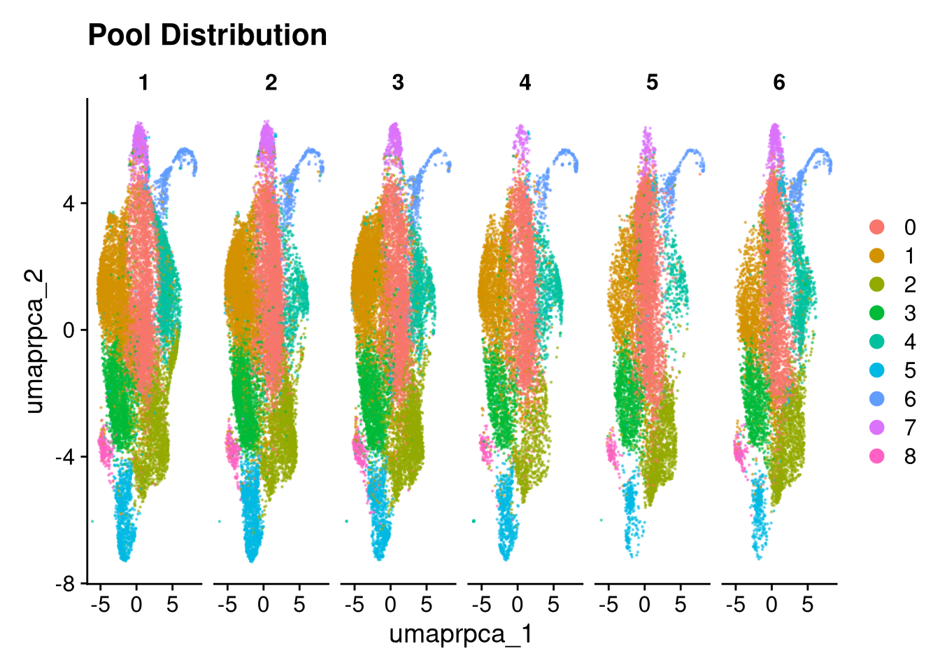
16:02:27 Optimization finishedp <- DimPlot(seu_h_f,
reduction = "umap",
split.by = "pool_id",
group.by = "pool_id") +
ggtitle("Unintegrated Data: Split by Pool")
p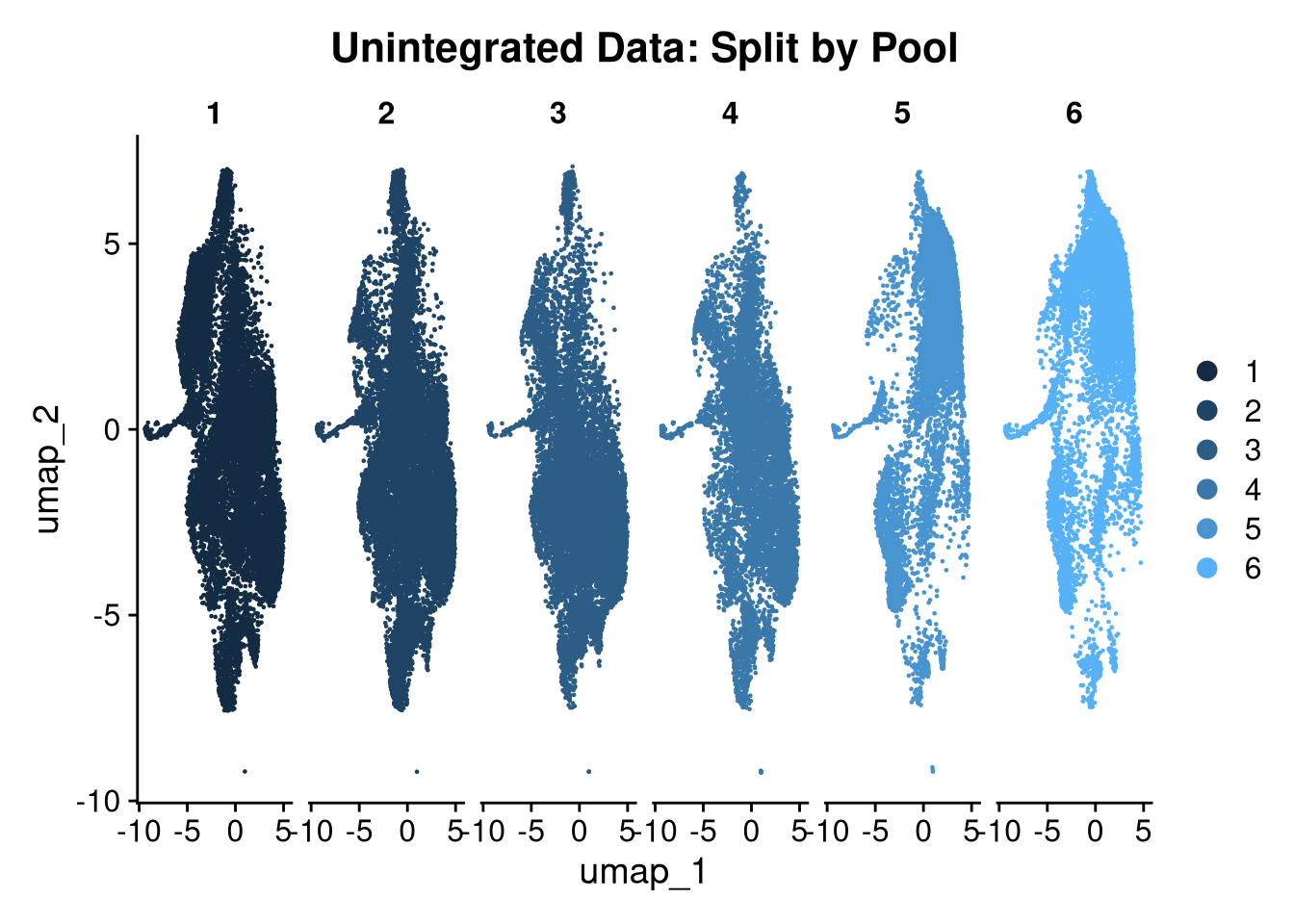
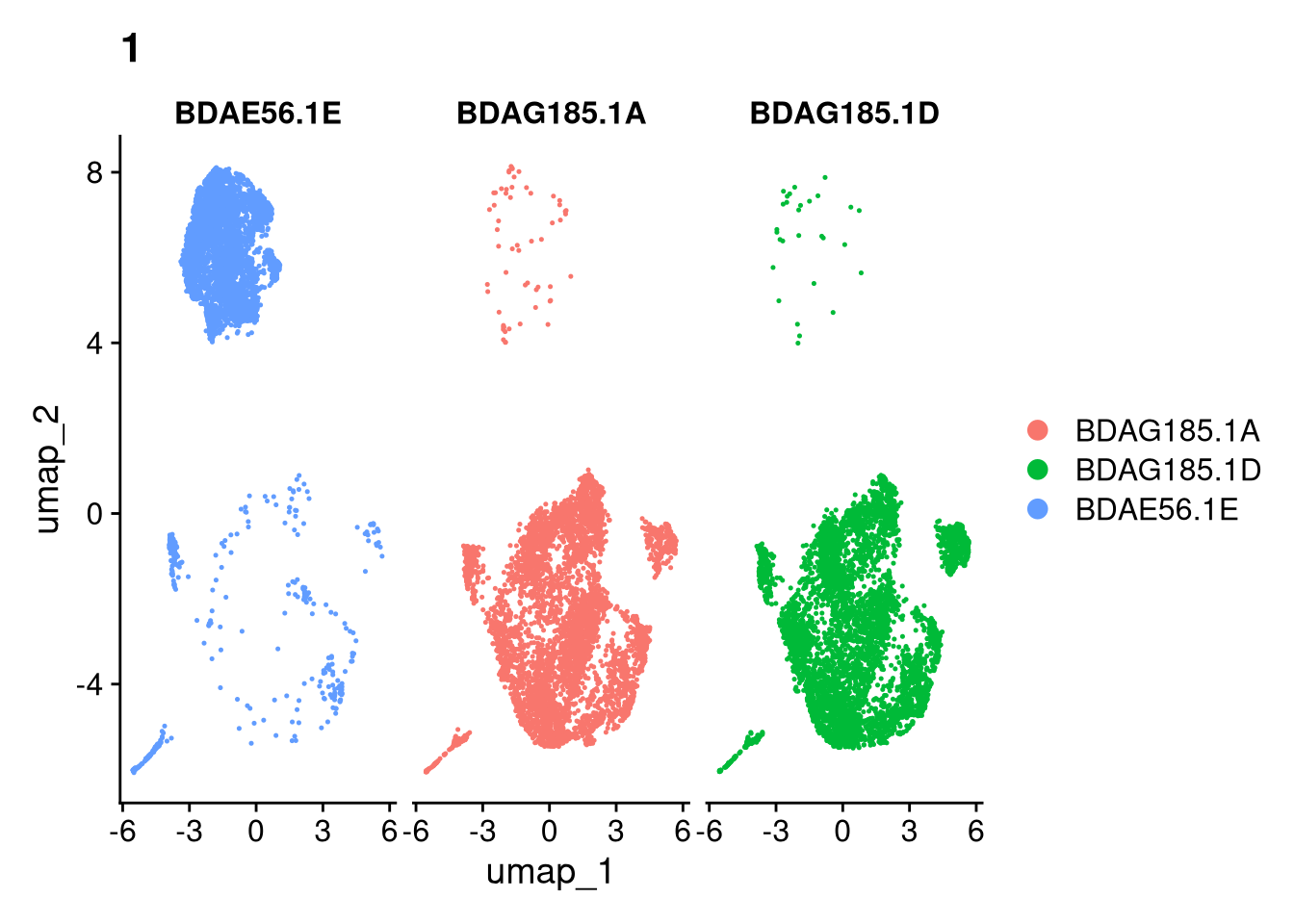
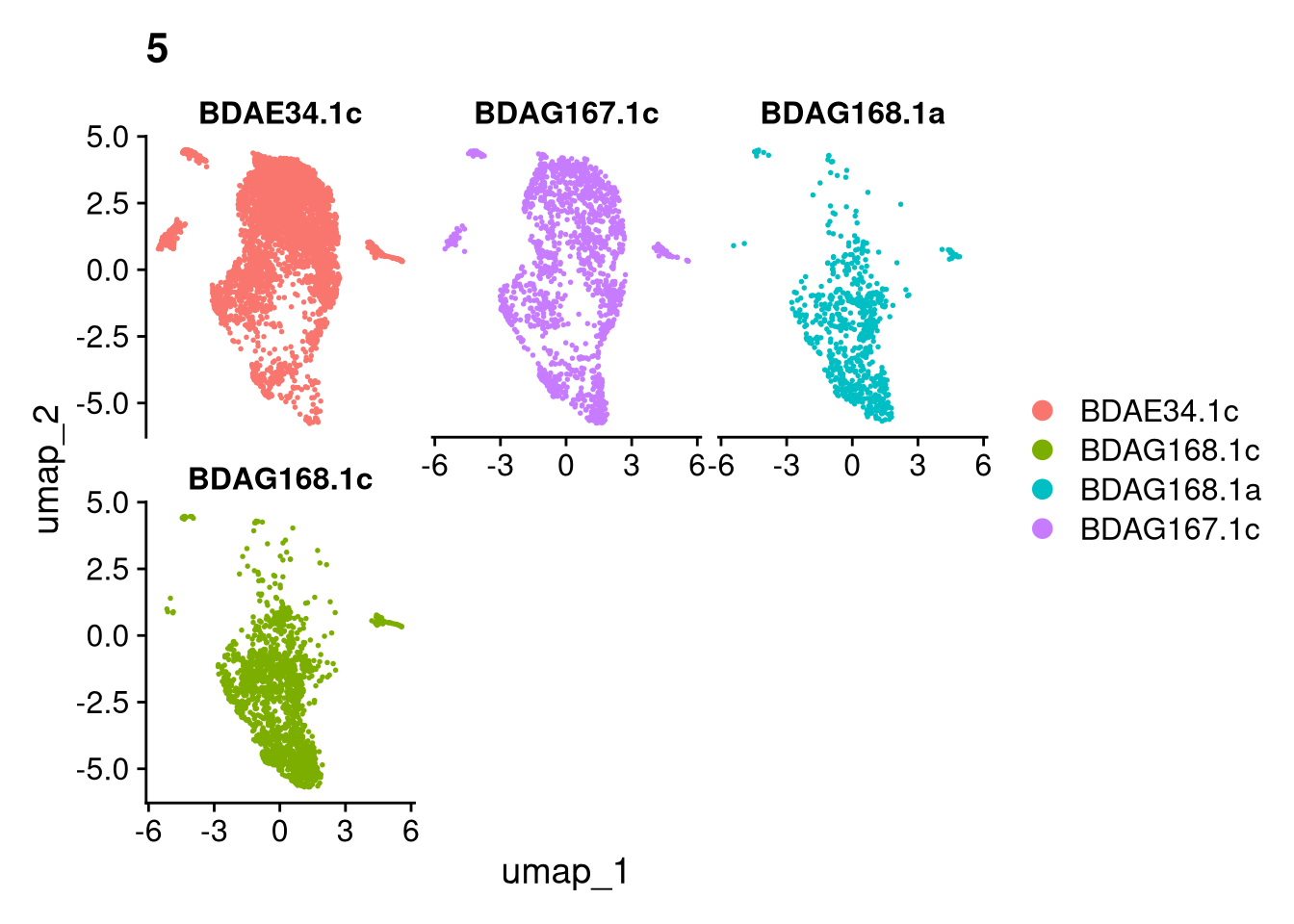
ggsave(file.path(graphs_dir, "QC_umaps_pools_split.pdf"), plot = p, width = 18, height = 6, units = "in")Each pool is processed independently to confirm quality on the clean data and re-score cell type identity before integration.
Gene sets for non-microglial cell types (provided by Emma) and Mancuso 2024 microglial states are loaded here for use in both batch-level and integrated scoring.
sig_dir <- file.path(base_dir, "signatures")
gs_myeloid <- readLines(file.path(sig_dir, "myeloid.txt"))
gs_proliferating <- readLines(file.path(sig_dir, "proliferating.txt"))
gs_macrophage <- readLines(file.path(sig_dir, "macrophage.txt"))
gs_dendritic <- readLines(file.path(sig_dir, "dendritic.txt"))
mancuso_dir <- "/nemo/lab/destrooperb/home/shared/zanettc/Mancuso2024_genesets"
gs_crm <- readLines(file.path(mancuso_dir, "CRM_geneset.txt"))
gs_dam <- readLines(file.path(mancuso_dir, "DAM_geneset.txt"))
gs_hla <- readLines(file.path(mancuso_dir, "HLA_geneset.txt"))
gs_hm <- readLines(file.path(mancuso_dir, "HM_geneset.txt"))
gs_irm <- readLines(file.path(mancuso_dir, "IRM_geneset.txt"))
gs_rm <- readLines(file.path(mancuso_dir, "RM_geneset.txt"))
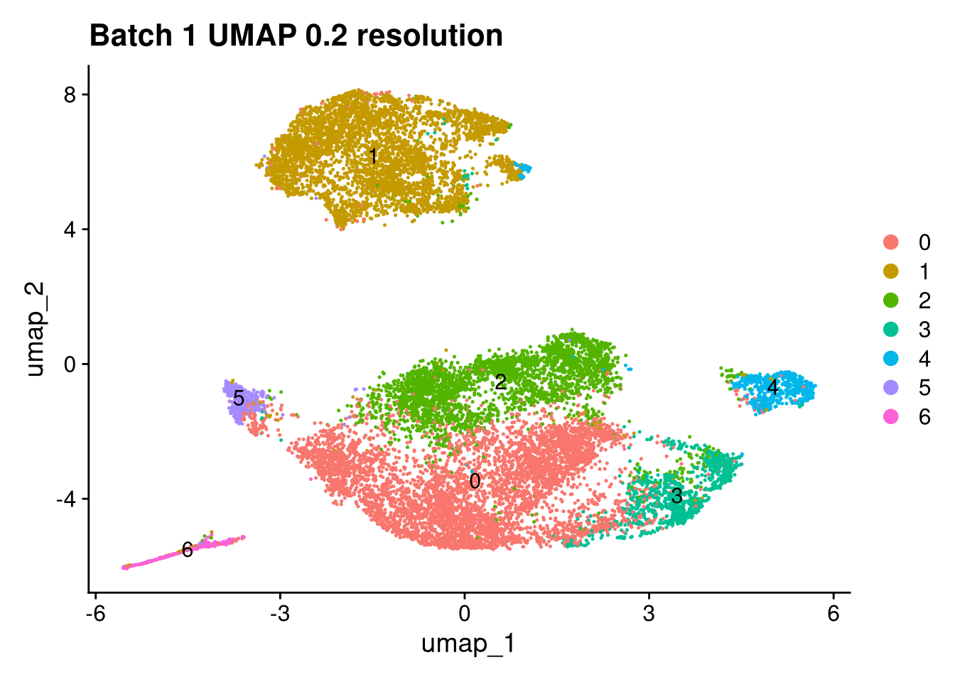
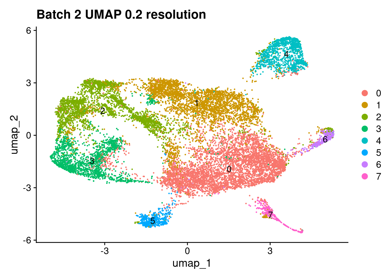
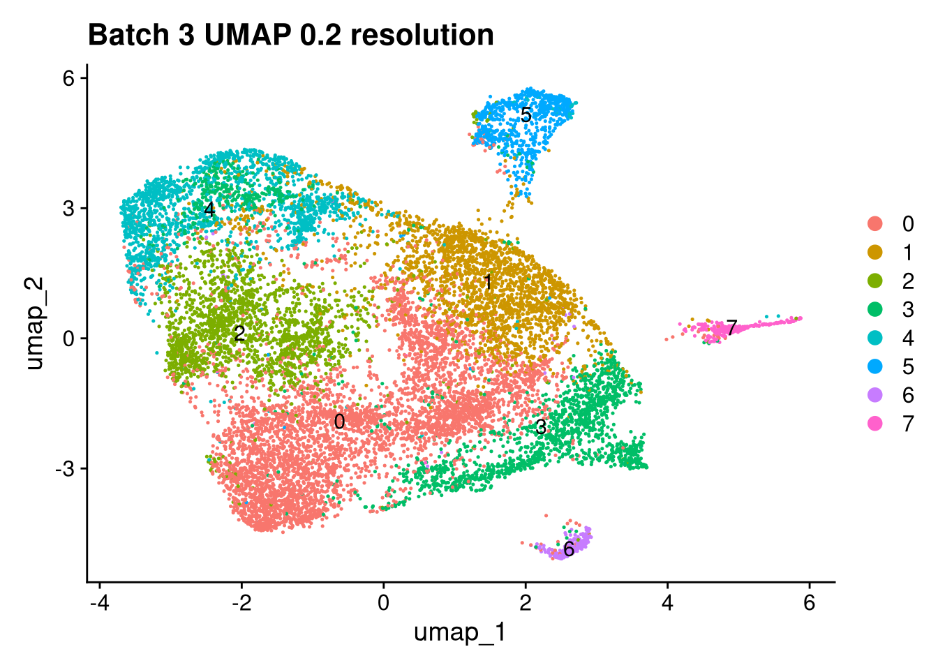
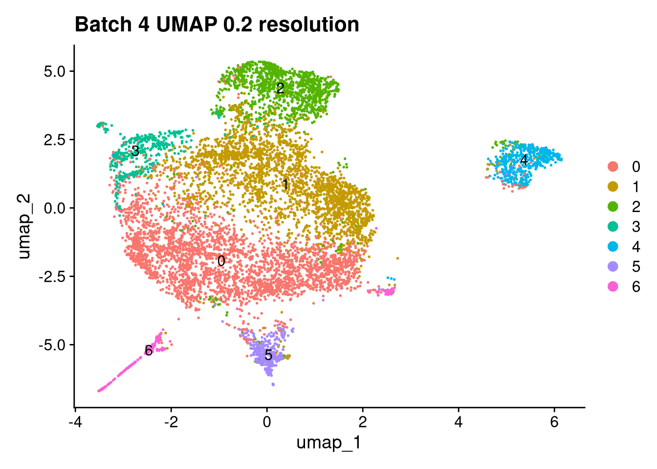
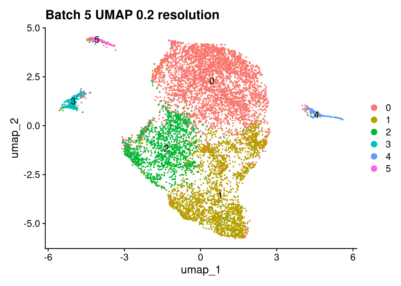
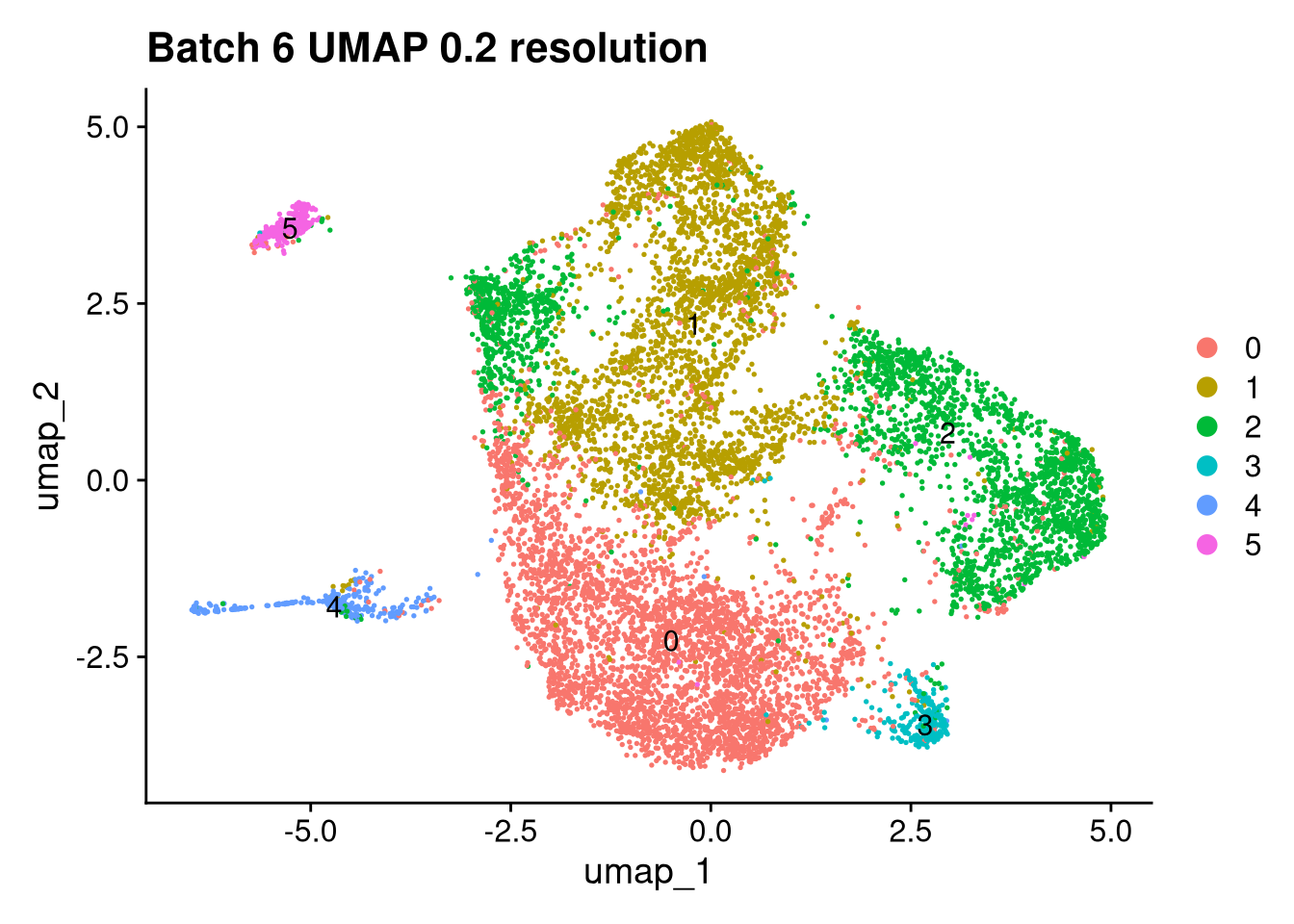
gs_tcrm <- readLines(file.path(mancuso_dir, "transCRM_geneset.txt"))Each batch is normalised with SCTransform, reduced with PCA, and embedded with UMAP. Clustering at resolution 0.2 generates initial cluster assignments for module scoring.
batches <- SplitObject(seu_h_f, split.by = "pool_id")
options(future.globals.maxSize = 8912896000000)
batches <- lapply(batches, SCTransform)
batches <- lapply(batches, \(o) {
set.seed(42)
o <- RunPCA(o, npcs = 30, assay = "SCT", verbose = FALSE)
set.seed(42)
o <- RunUMAP(o, dims = 1:25, n.neighbors = 30L, n.epochs = 500, min.dist = 0.05)
o
})
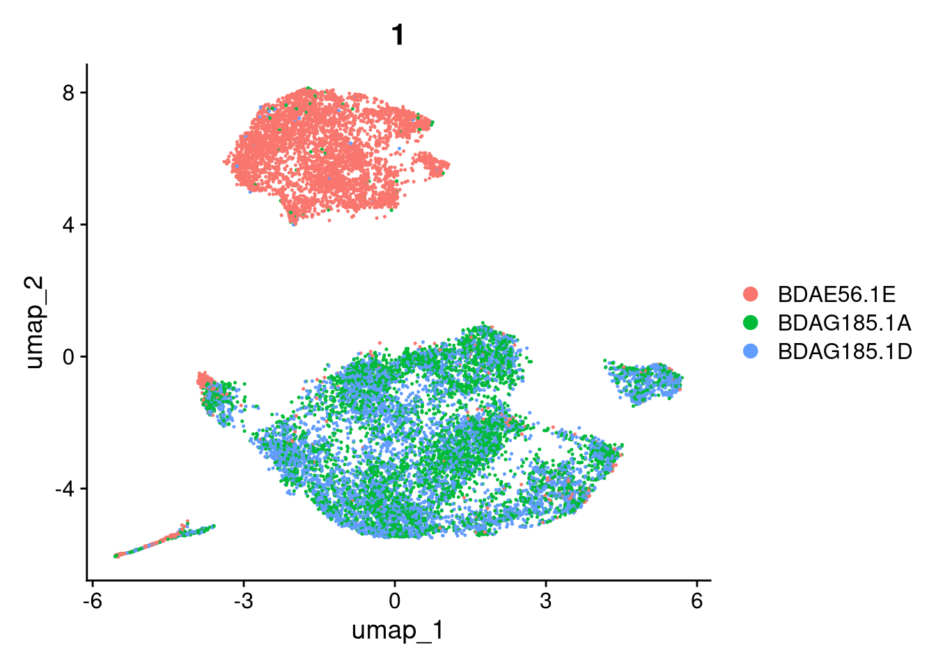
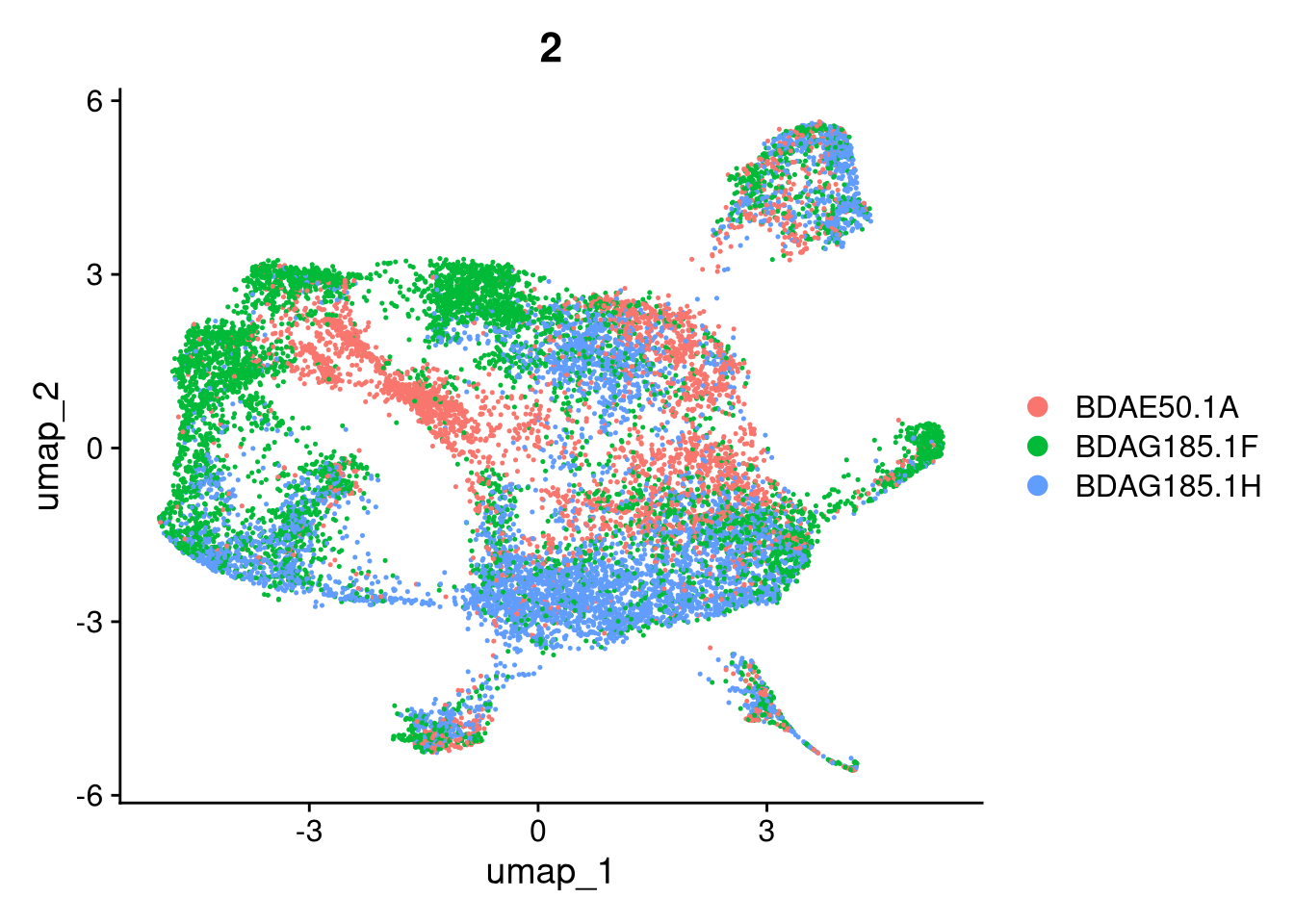
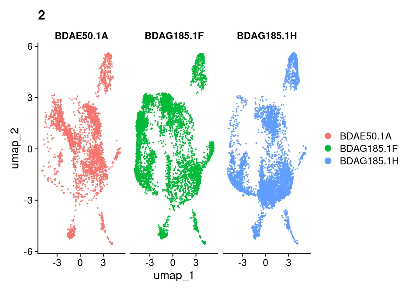
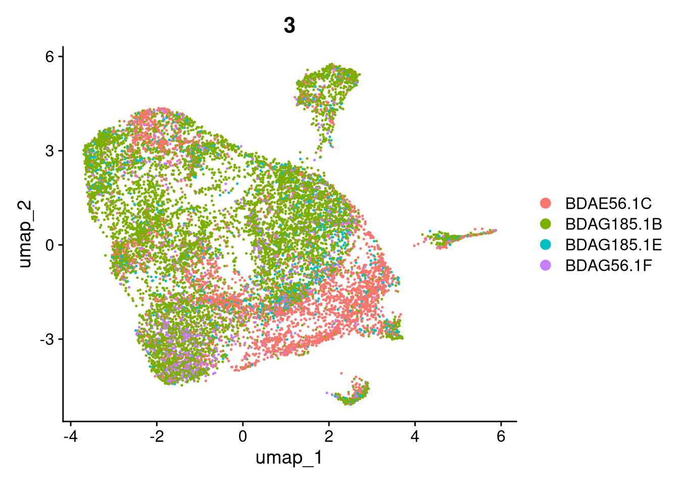
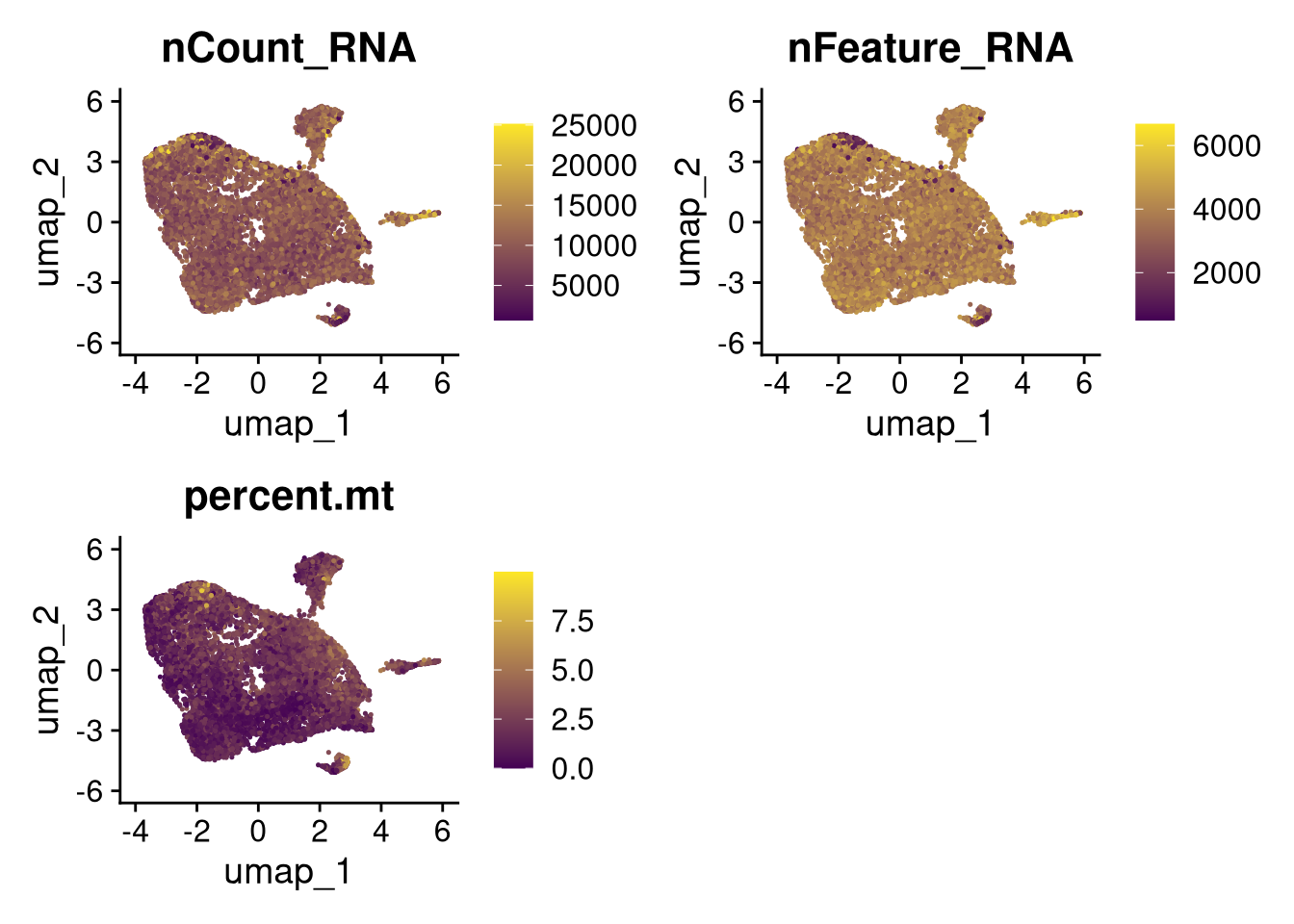
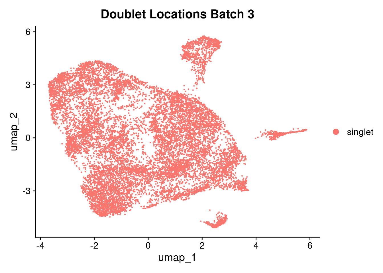
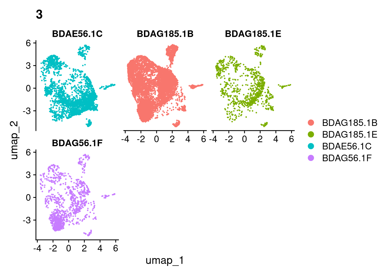
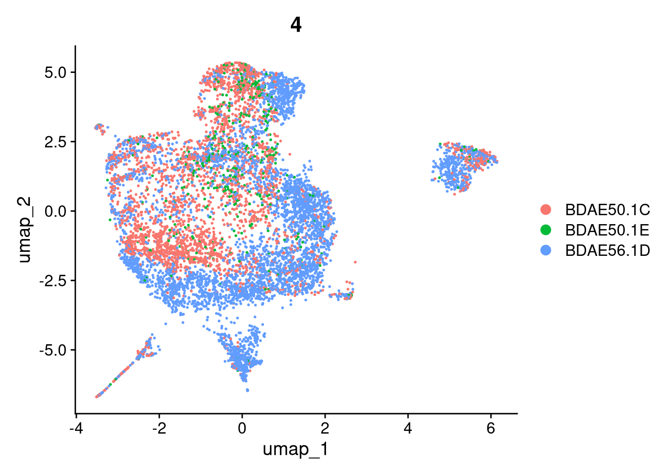
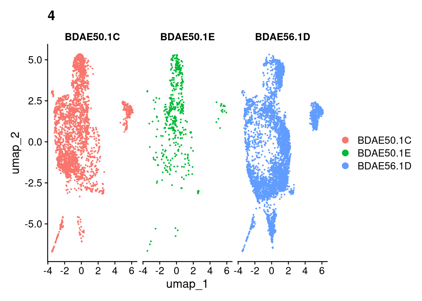
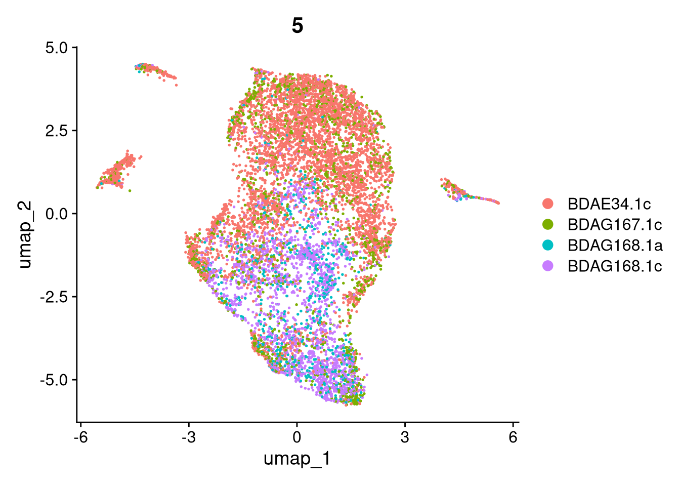
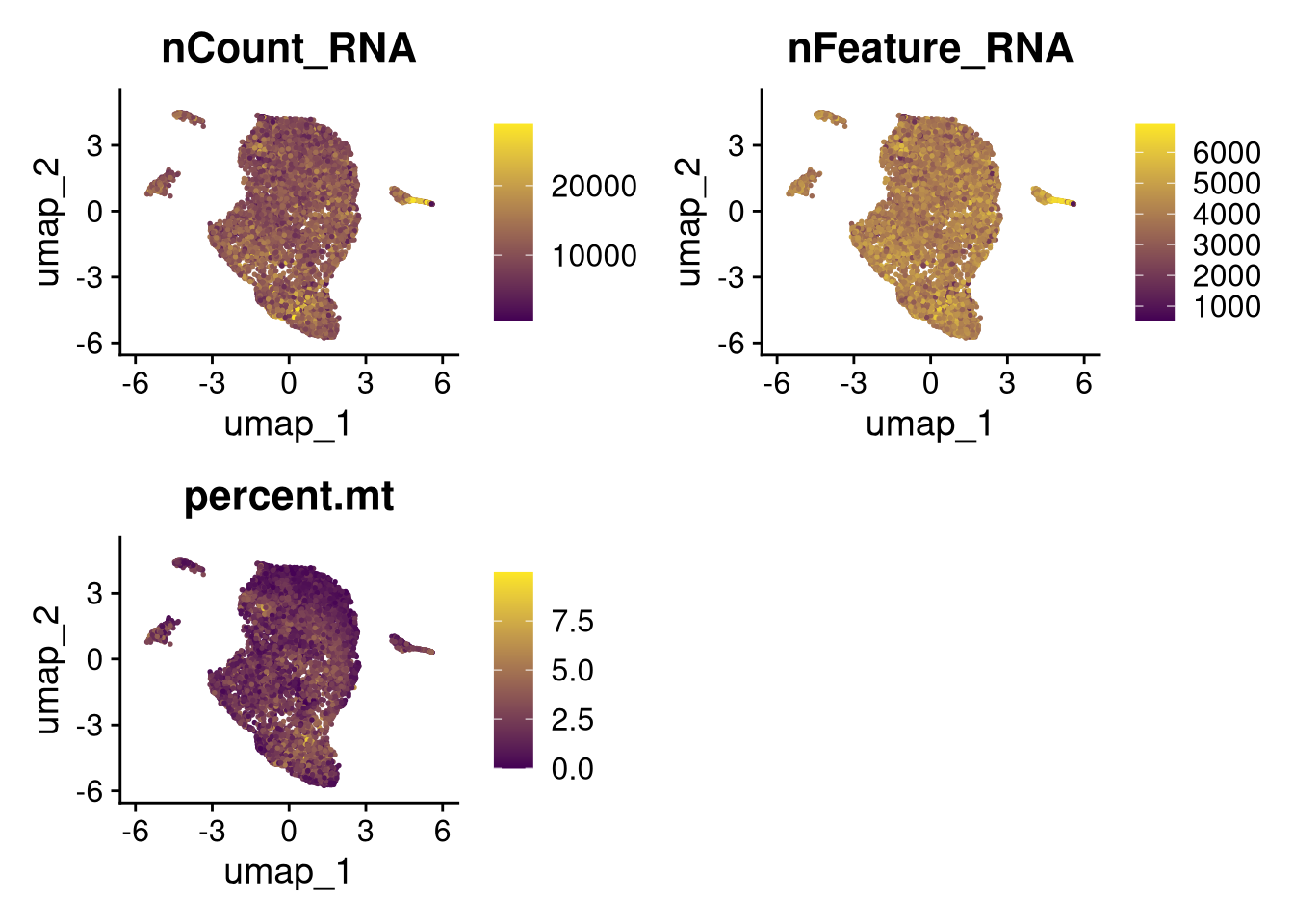
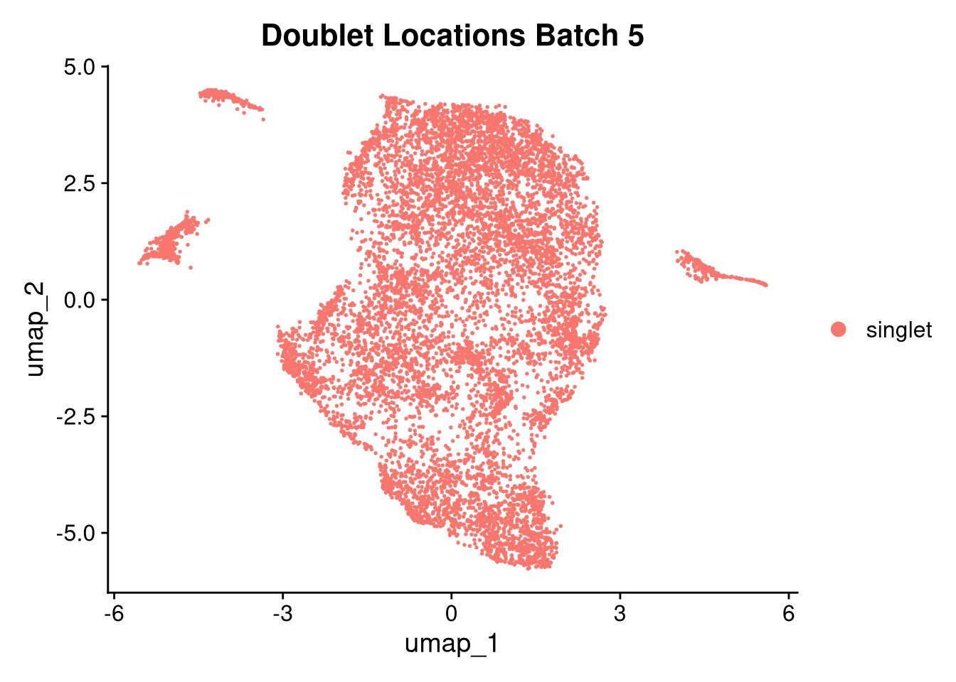
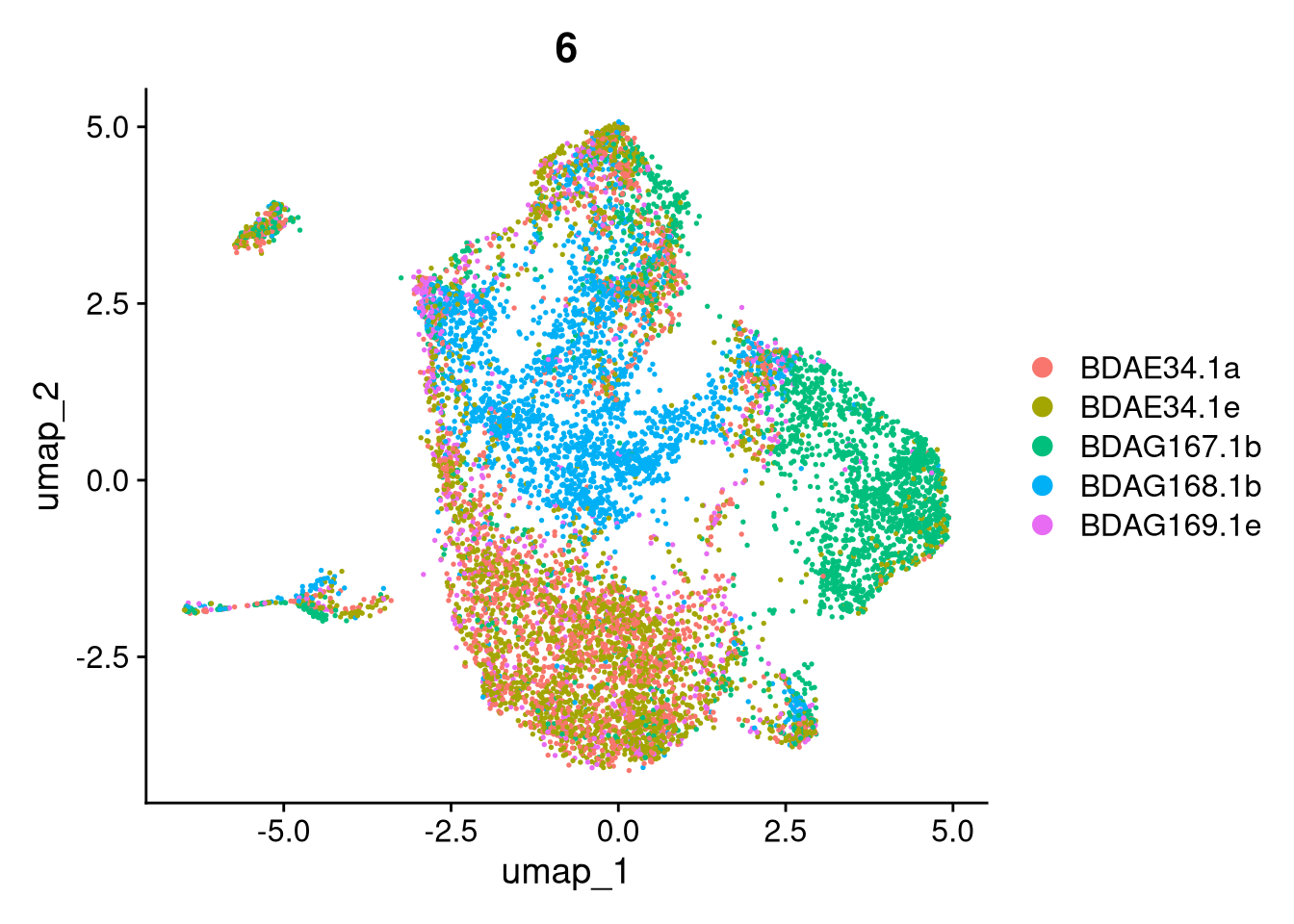
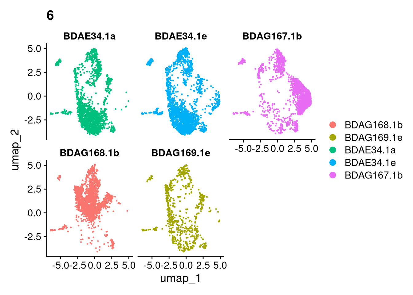
invisible(lapply(names(batches), function(nm) {
p <- DimPlot(batches[[nm]], reduction = "umap", group.by = "orig.ident", shuffle = TRUE) + ggtitle(nm)
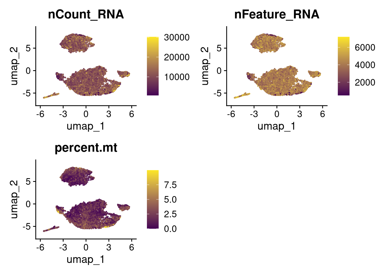
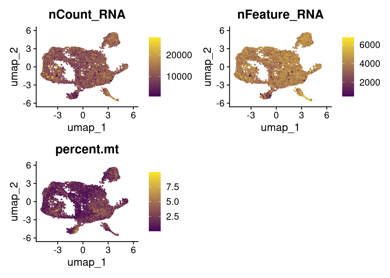
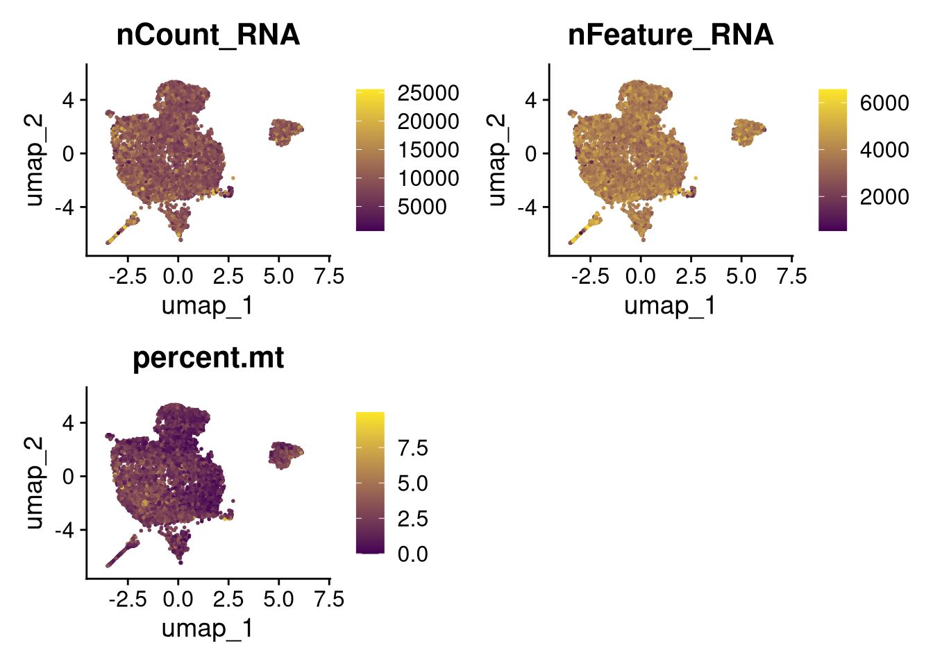
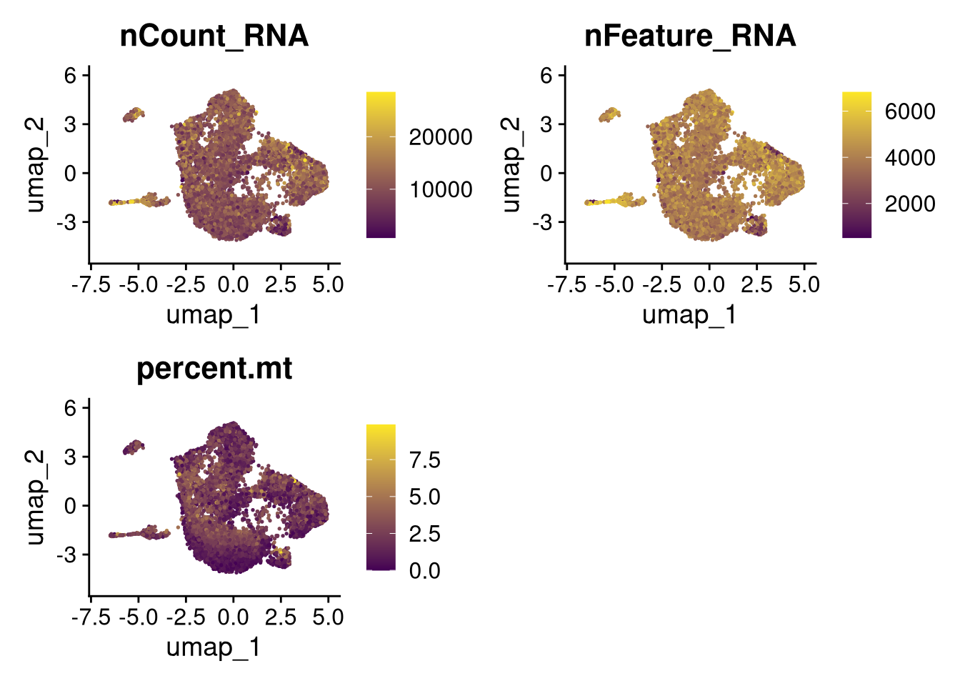
p2 <- FeaturePlot(batches[[nm]], features = c("nCount_RNA", "nFeature_RNA", "percent.mt"), cols = c("#440154", "#FDE725"))
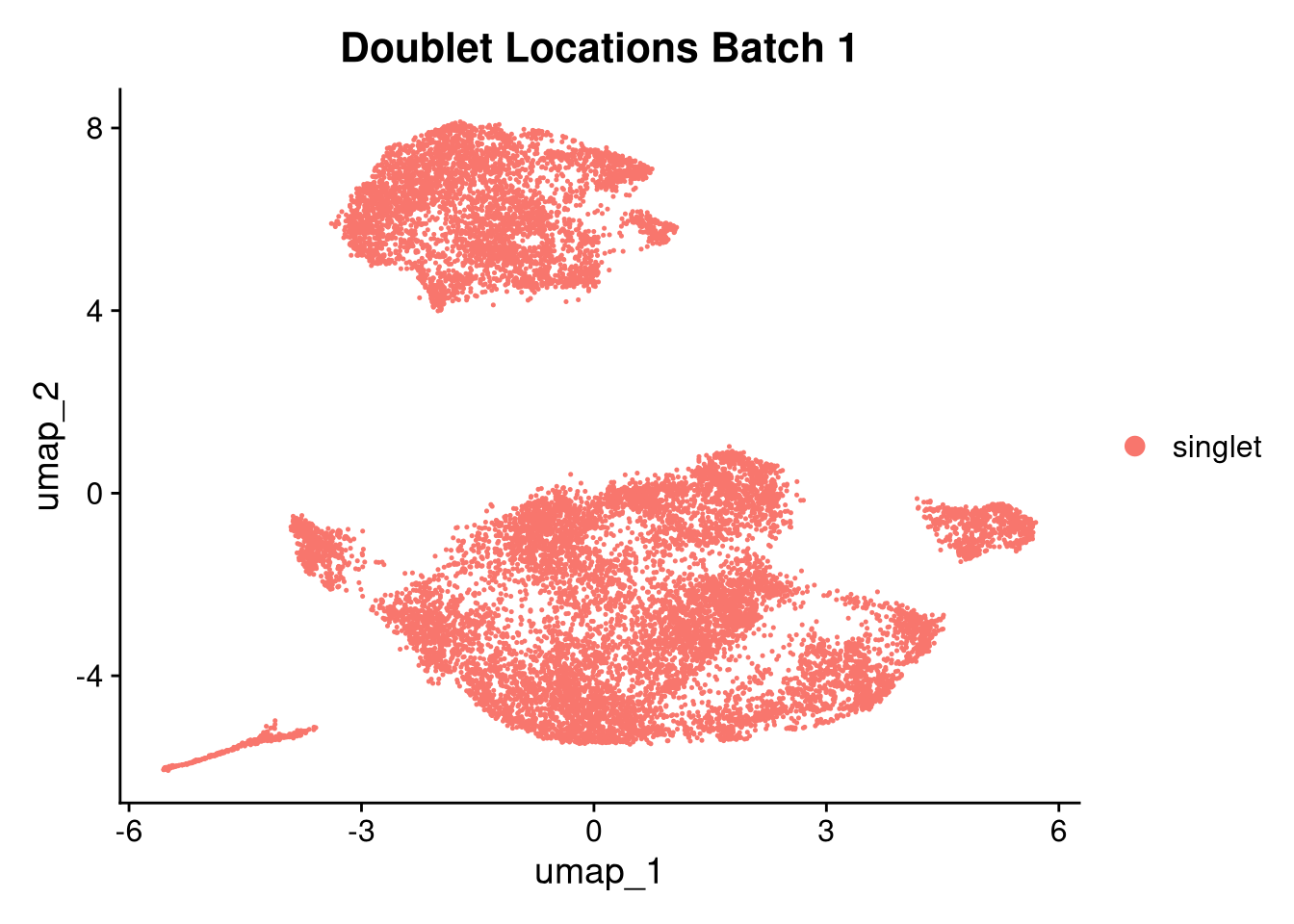
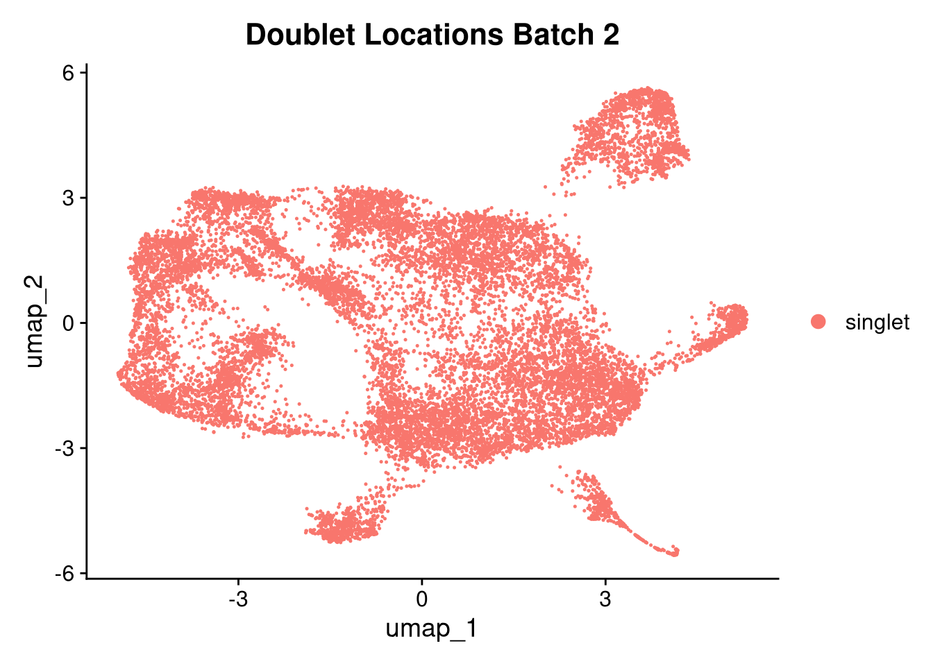
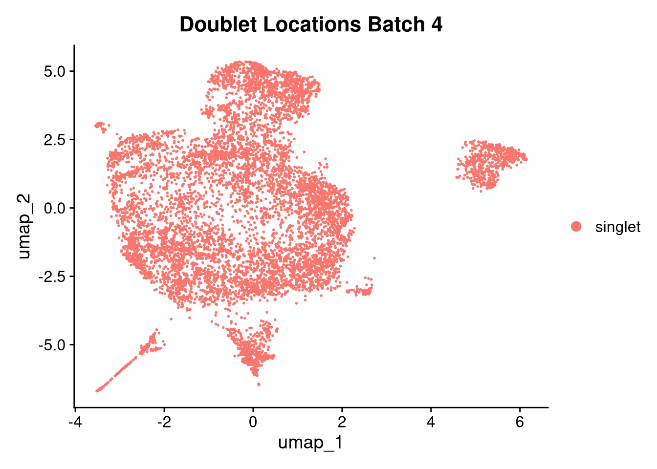
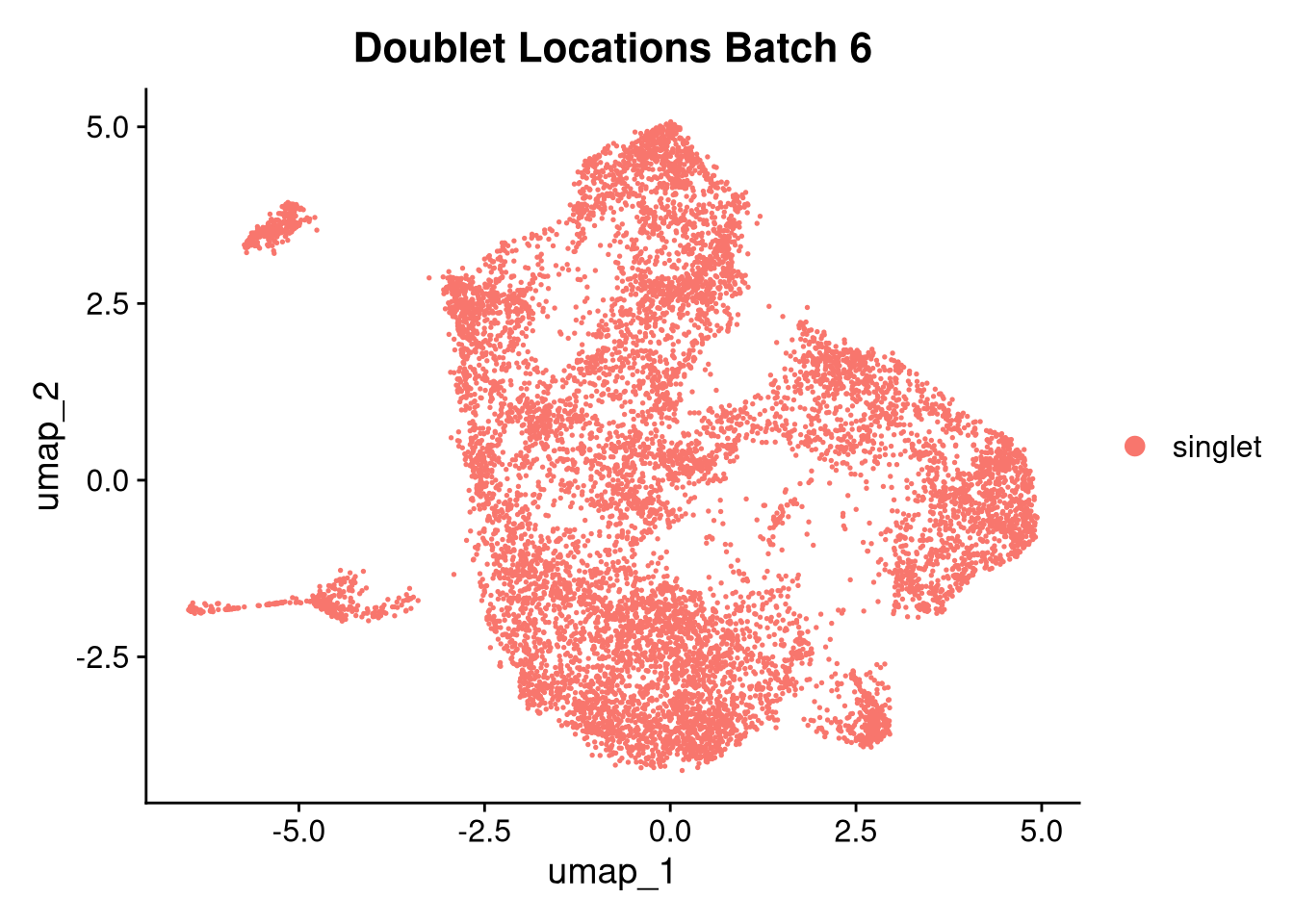
p3 <- DimPlot(batches[[nm]], group.by = "scDblFinder.class") + ggtitle(glue("Doublet Locations Batch {nm}"))
p4 <- DimPlot(batches[[nm]], reduction = "umap", split.by = "orig.ident", shuffle = TRUE, ncol = 3) + ggtitle(nm)
print(p); print(p2); print(p3); print(p4)
batch_graphs_dir <- file.path(graphs_dir, glue("batch_{nm}"))
dir.create(batch_graphs_dir, recursive = TRUE, showWarnings = FALSE)
ggsave(filename = file.path(batch_graphs_dir, glue("QC_batch{nm}_umap_samples_overlayed.pdf")), plot = p, width = 7, height = 5, dpi = 300, units = "in")
ggsave(filename = file.path(batch_graphs_dir, glue("QC_batch{nm}_umap_qc_x3.pdf")), plot = p2, width = 7, height = 5, dpi = 300, units = "in")
ggsave(filename = file.path(batch_graphs_dir, glue("QC_batch{nm}_doublets_umap.pdf")), plot = p3, width = 7, height = 5, dpi = 300, units = "in")
ggsave(filename = file.path(batch_graphs_dir, glue("QC_batch{nm}_umap_samples_split.pdf")), plot = p4, width = 7, height = 5, dpi = 300, units = "in")
}))
qs_save(batches, file = file.path(objects_dir, "umap_batches.qs2"))batches <- qs_read(file.path(objects_dir, "umap_batches.qs2"))res <- 0.2
batches <- lapply(batches, \(o) {
set.seed(42)
o <- FindNeighbors(o, reduction = "pca", dims = 1:30)
set.seed(42)
o <- FindClusters(o, resolution = res)
})Modularity Optimizer version 1.3.0 by Ludo Waltman and Nees Jan van Eck
Number of nodes: 15782
Number of edges: 529123
Running Louvain algorithm...
Maximum modularity in 10 random starts: 0.9016
Number of communities: 7
Elapsed time: 2 secondsModularity Optimizer version 1.3.0 by Ludo Waltman and Nees Jan van Eck
Number of nodes: 15812
Number of edges: 538867
Running Louvain algorithm...
Maximum modularity in 10 random starts: 0.8947
Number of communities: 8
Elapsed time: 2 secondsModularity Optimizer version 1.3.0 by Ludo Waltman and Nees Jan van Eck
Number of nodes: 14074
Number of edges: 448048
Running Louvain algorithm...
Maximum modularity in 10 random starts: 0.8671
Number of communities: 8
Elapsed time: 2 secondsModularity Optimizer version 1.3.0 by Ludo Waltman and Nees Jan van Eck
Number of nodes: 8488
Number of edges: 291700
Running Louvain algorithm...
Maximum modularity in 10 random starts: 0.8749
Number of communities: 7
Elapsed time: 1 secondsModularity Optimizer version 1.3.0 by Ludo Waltman and Nees Jan van Eck
Number of nodes: 9255
Number of edges: 302324
Running Louvain algorithm...
Maximum modularity in 10 random starts: 0.8681
Number of communities: 6
Elapsed time: 1 secondsModularity Optimizer version 1.3.0 by Ludo Waltman and Nees Jan van Eck
Number of nodes: 10456
Number of edges: 347686
Running Louvain algorithm...
Maximum modularity in 10 random starts: 0.8813
Number of communities: 6
Elapsed time: 1 secondsinvisible(lapply(names(batches), function(nm) {
p <- DimPlot(batches[[nm]], reduction = "umap", label = TRUE) +
ggtitle(glue("Batch {nm} UMAP {res} resolution"))
print(p)
batch_graphs_dir <- file.path(graphs_dir, glue("batch_{nm}"))
ggsave(
filename = file.path(batch_graphs_dir, glue("clusters_batch_{nm}_{res}.pdf")),
plot = p, width = 7, height = 5, dpi = 300, units = "in"
)
}))
for (i in seq_along(batches)) {
  qs_save(batches[[i]], file = paste0(objects_dir, "/batch", i, "_clustered.qs2"))
}files <- list.files(path = objects_dir, pattern = "batch[0-9]+_clustered.qs2", full.names = TRUE)
batches <- lapply(files, qs_read)Gene sets are intersected against the batch feature space before scoring. AddModuleScore calculates average expression of each gene set relative to a randomly sampled control set, giving a background-corrected enrichment score per cell.
myeloid_seu <- intersect(gs_myeloid, rownames(batches[[1]]))
prolif_seu <- intersect(gs_proliferating, rownames(batches[[1]]))
macrophage_seu <- intersect(gs_macrophage, rownames(batches[[1]]))
dendritic_seu <- intersect(gs_dendritic, rownames(batches[[1]]))
gene_sets <- list(
dendritic = dendritic_seu,
proliferating = prolif_seu,
macrophage = macrophage_seu,
myeloid = myeloid_seu,
CRM = gs_crm,
DAM = gs_dam,
HLA = gs_hla,
HM = gs_hm,
IRM = gs_irm,
RM = gs_rm,
tCRM = gs_tcrm
)
batches <- lapply(seq_along(batches), function(i) {
o <- batches[[i]]
nm <- as.character(i)
message(glue("Processing Batch {nm}..."))
batch_graphs_dir <- file.path(graphs_dir, glue("batch_{nm}"))
if (!dir.exists(batch_graphs_dir)) dir.create(batch_graphs_dir, recursive = TRUE)
o <- AddModuleScore(object = o, features = gene_sets, name = names(gene_sets), ctrl = 5, seed = 42)
o$seurat_clusters <- factor(
o$seurat_clusters,
levels = sort(as.numeric(unique(as.character(o$seurat_clusters))))
)
Idents(o) <- "seurat_clusters"
p1 <- VlnPlot(o, features = c("dendritic1", "proliferating2", "macrophage3", "myeloid4"),
group.by = "seurat_clusters", pt.size = 0, ncol = 2) +
ggtitle(glue("Batch {nm}: Cell Types"))
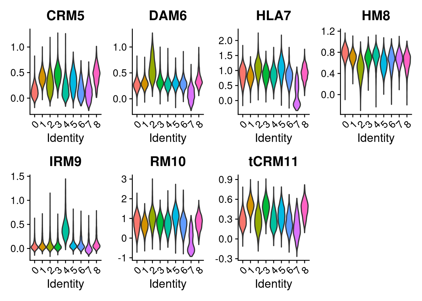
p2 <- VlnPlot(o, features = c("CRM5", "DAM6", "HLA7", "HM8", "IRM9", "RM10", "tCRM11"),
group.by = "seurat_clusters", pt.size = 0, ncol = 4) +
ggtitle(glue("Batch {nm}: Mancuso Scores"))
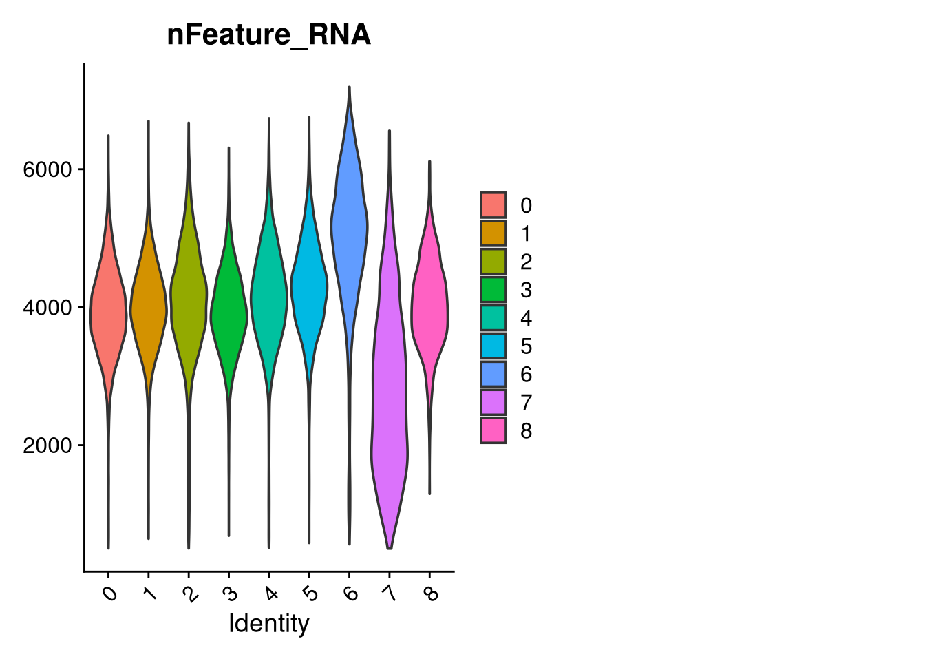
p3 <- VlnPlot(o, features = c("nFeature_RNA"),
group.by = "seurat_clusters", pt.size = 0, ncol = 2) +
ggtitle(glue("Batch {nm}: QC"))
ggsave(filename = file.path(batch_graphs_dir, glue("batch_{nm}_celltypes.pdf")), plot = p1, width = 7, height = 5, dpi = 300)
ggsave(filename = file.path(batch_graphs_dir, glue("batch_{nm}_mancuso.pdf")), plot = p2, width = 10, height = 5, dpi = 300)
ggsave(filename = file.path(batch_graphs_dir, glue("batch_{nm}_qc.pdf")), plot = p3, width = 10, height = 5, dpi = 300)
return(o)
})Batches are merged back into a single object and re-normalised with SCTransform v2. PCA is run on the merged, unintegrated object to provide the input embedding required by RPCA. Integration with IntegrateLayers (RPCA method) corrects pool-level batch effects while aiming to preserve biological variance.
merged_obj <- merge(batches[[1]], y = batches[-1])
Idents(merged_obj) <- "pool_id"

options(future.globals.maxSize = 100 * 1024^3)
merged_obj <- SCTransform(merged_obj, vst.flavor = "v2", verbose = FALSE)
merged_obj <- RunPCA(merged_obj, verbose = FALSE, assay = "SCT")

set.seed(42)
int_method <- "rpca"
DefaultAssay(merged_obj) <- "SCT"
merged_obj <- IntegrateLayers(
  object               = merged_obj,
  method               = RPCAIntegration,
  normalization.method = "SCT",
  orig.reduction       = "pca",
  new.reduction        = glue("integrated.{int_method}"),
  verbose              = FALSE
)Neighbours are found on the integrated RPCA reduction and clusters are identified at resolution 0.15. A UMAP is computed on the same integrated reduction for visualisation.
set.seed(42)
merged_obj <- FindNeighbors(merged_obj, reduction = glue("integrated.{int_method}"), dims = 1:30)

set.seed(42)
cluster_resolution <- 0.15
merged_obj <- FindClusters(
  merged_obj,
  resolution   = cluster_resolution,
  cluster.name = glue("{int_method}_clusters"),
  graph.name   = "SCT_snn"
)
Modularity Optimizer version 1.3.0 by Ludo Waltman and Nees Jan van Eck
Number of nodes: 73867
Number of edges: 2347692
Running Louvain algorithm...
Maximum modularity in 10 random starts: 0.9227
Number of communities: 9
Elapsed time: 37 secondsset.seed(42)
merged_obj <- RunUMAP(
merged_obj,
dims = 1:30,
reduction.name = glue("umap.{int_method}")
)16:28:40 UMAP embedding parameters a = 0.9922 b = 1.11216:28:40 Read 73867 rows and found 30 numeric columns16:28:40 Using Annoy for neighbor search, n_neighbors = 3016:28:40 Building Annoy index with metric = cosine, n_trees = 500% 10 20 30 40 50 60 70 80 90 100%[----|----|----|----|----|----|----|----|----|----|**************************************************|
16:28:45 Writing NN index file to temp file /tmp/slurm_46128766/RtmppchOMW/file3ec1ba62834870
16:28:45 Searching Annoy index using 1 thread, search_k = 3000
16:29:13 Annoy recall = 100%
16:29:15 Commencing smooth kNN distance calibration using 1 thread with target n_neighbors = 30
16:29:20 Initializing from normalized Laplacian + noise (using RSpectra)
16:29:24 Commencing optimization for 200 epochs, with 3362430 positive edges
16:29:24 Using rng type: pcg
16:29:58 Optimization finishedqs_save(merged_obj, file = file.path(objects_dir, "prelabelled_integrated_rpca.qs2"))
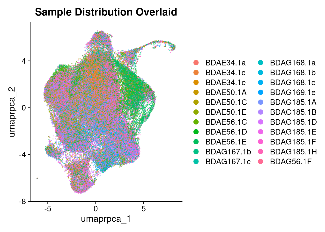
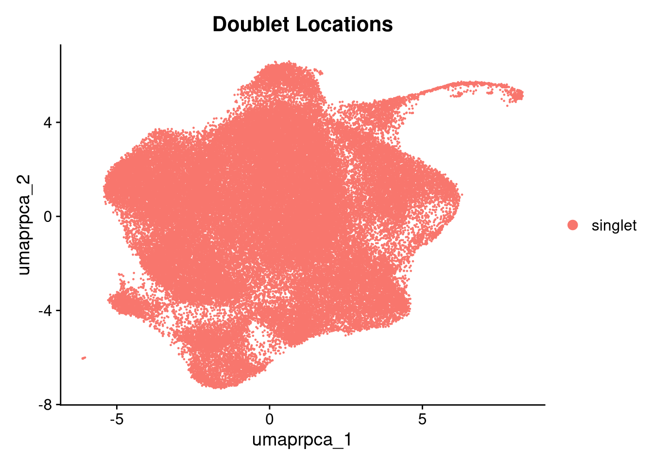
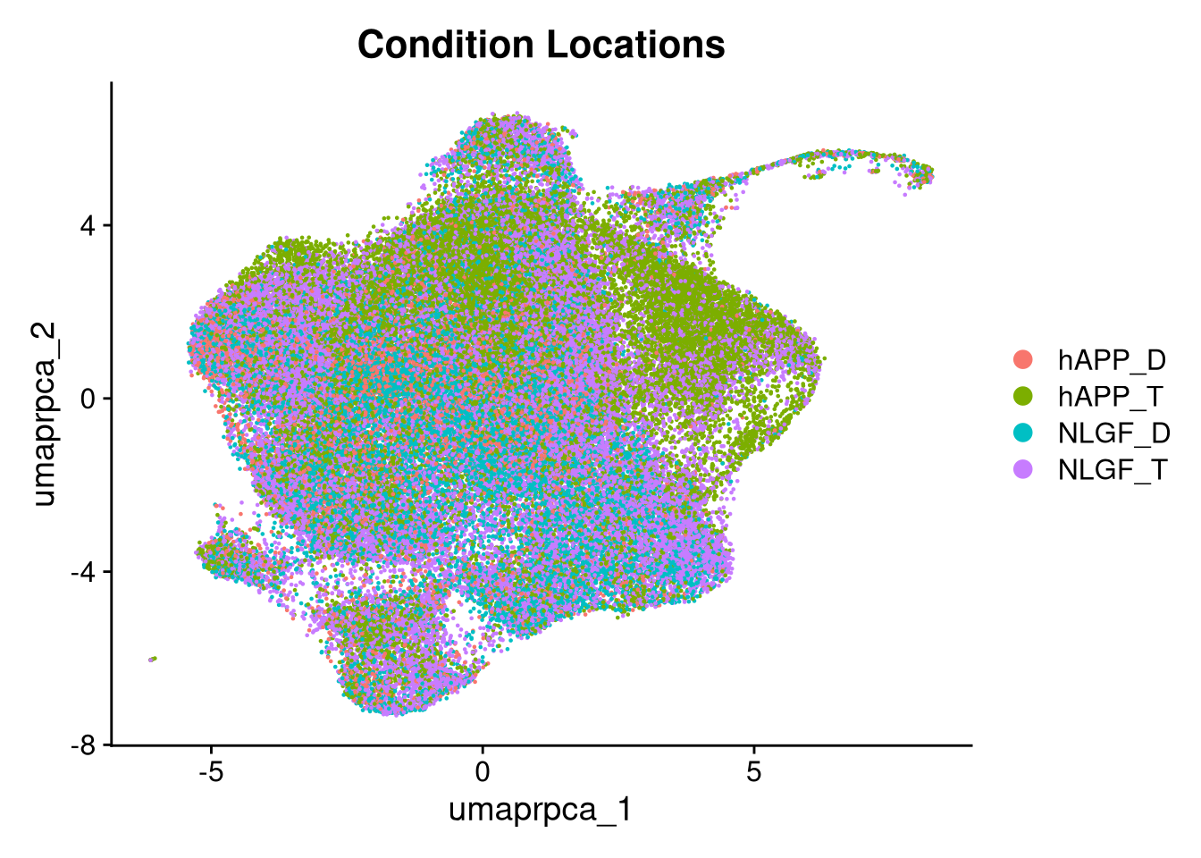
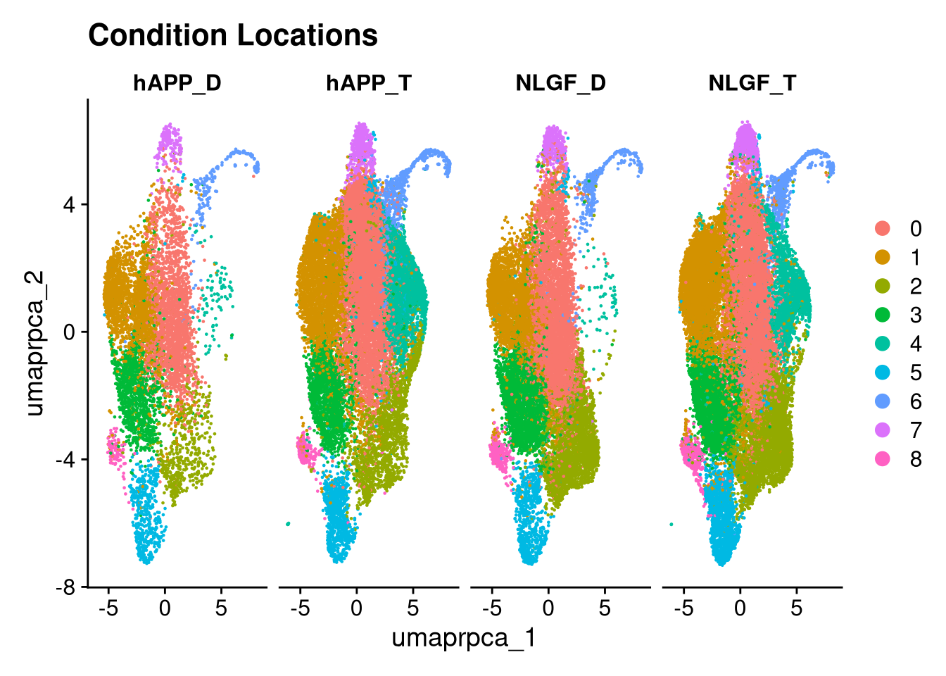
merged_obj <- qs_read(file.path(objects_dir, "prelabelled_integrated_rpca.qs2"))A standard set of diagnostic plots checks cluster structure, sample and pool mixing, QC metric distributions, doublet and outlier locations, and condition separation.
p1 <- DimPlot(merged_obj, reduction = glue("umap.{int_method}"),
group.by = glue("{int_method}_clusters"), label = TRUE) +
ggtitle(glue("Clusters {cluster_resolution} resolution"))
p2 <- DimPlot(merged_obj, reduction = glue("umap.{int_method}"),
group.by = "orig.ident", shuffle = TRUE, alpha = 0.5) +
ggtitle("Sample Distribution Overlaid")
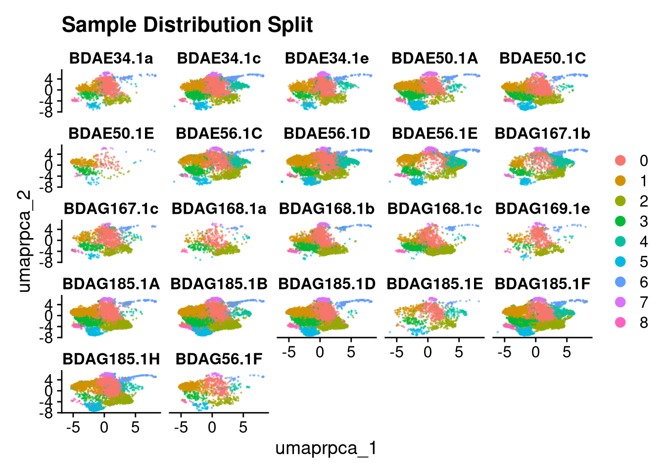
p2.5 <- DimPlot(merged_obj, reduction = glue("umap.{int_method}"),
split.by = "orig.ident", ncol = 5, alpha = 0.5) +
ggtitle("Sample Distribution Split")
p3 <- DimPlot(merged_obj, reduction = glue("umap.{int_method}"),
group.by = "pool_id", shuffle = TRUE, alpha = 0.5) +
ggtitle("Pool Distribution")
p3.5 <- DimPlot(merged_obj, reduction = glue("umap.{int_method}"),
split.by = "pool_id", shuffle = TRUE, alpha = 0.5) +
ggtitle("Pool Distribution")
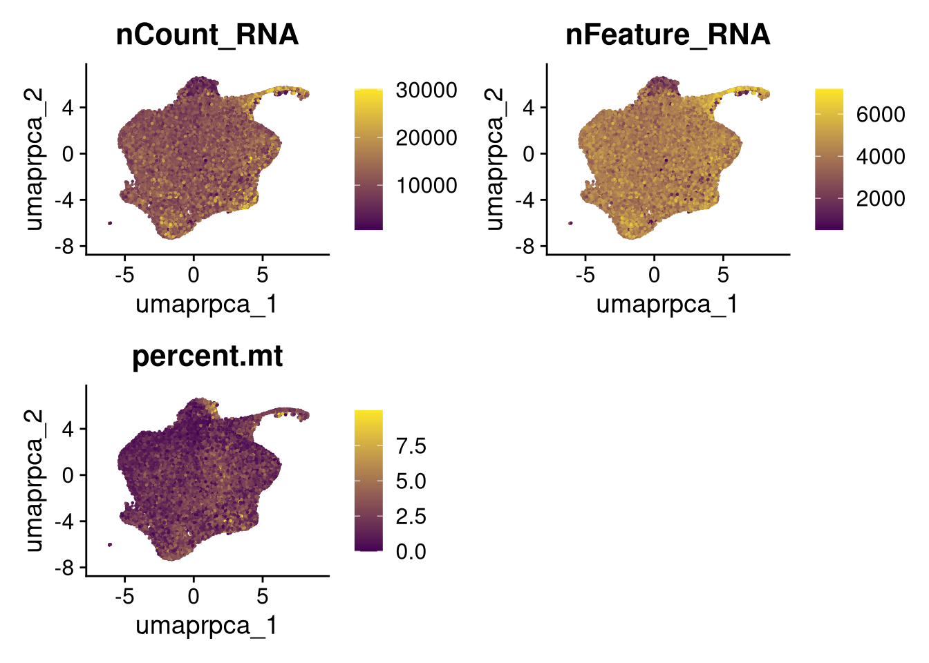
p4 <- FeaturePlot(merged_obj, reduction = glue("umap.{int_method}"),
features = c("nCount_RNA", "nFeature_RNA", "percent.mt"),
cols = c("#440154", "#FDE725"))
p5 <- DimPlot(merged_obj, reduction = glue("umap.{int_method}"),
group.by = "scDblFinder.class") +
ggtitle("Doublet Locations")
p5.5 <- DimPlot(merged_obj, reduction = glue("umap.{int_method}"),
group.by = "mad3_outlier") +
ggtitle("MAD3 Outlier Locations")
p6 <- DimPlot(merged_obj, reduction = glue("umap.{int_method}"),
group.by = "group_id", shuffle = TRUE) +
ggtitle("Condition Locations")
p6.5 <- DimPlot(merged_obj, reduction = glue("umap.{int_method}"),
split.by = "group_id", ncol = 5) +
ggtitle("Condition Locations")
print(p1); print(p2); print(p2.5)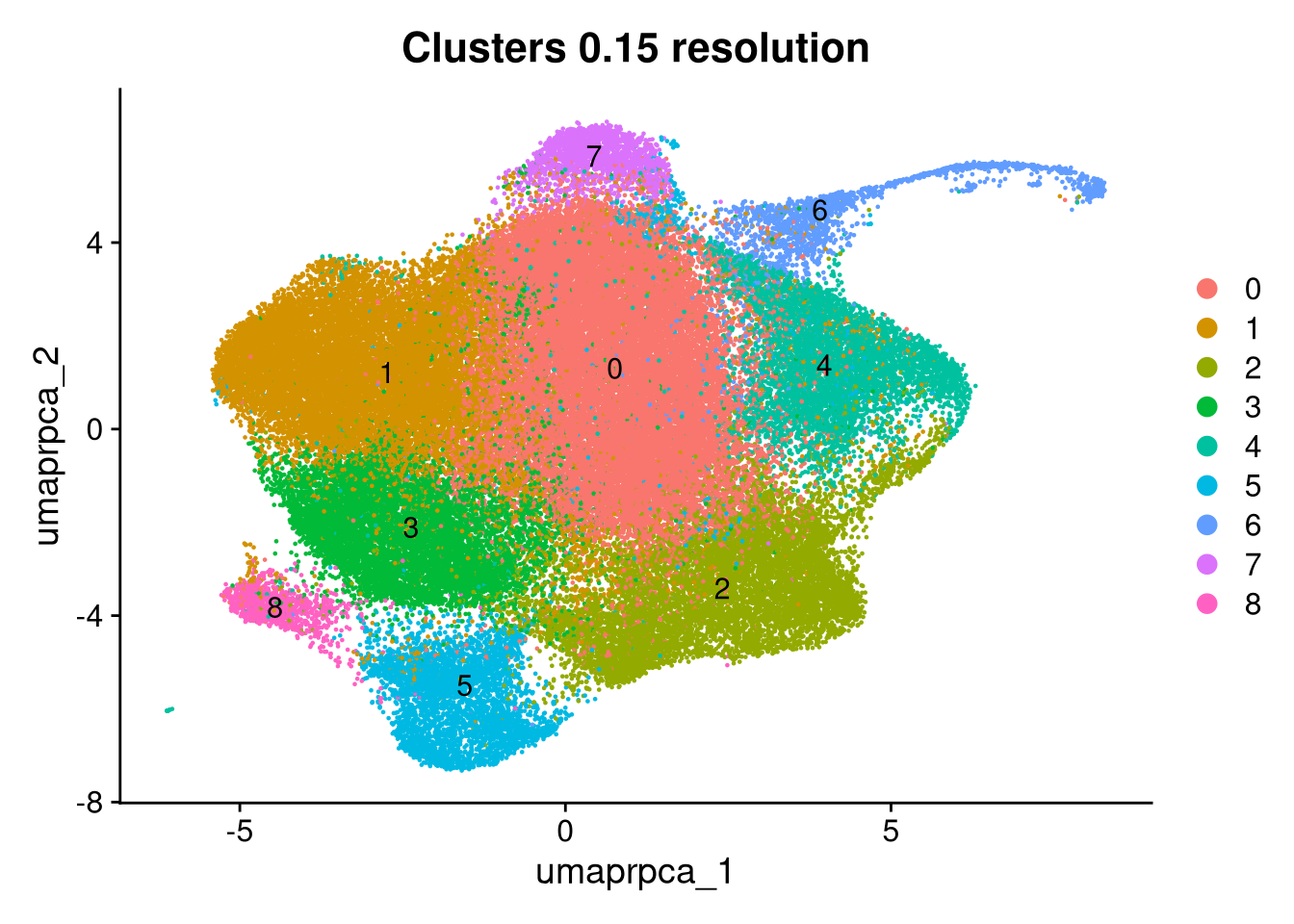
print(p3); print(p4); print(p5)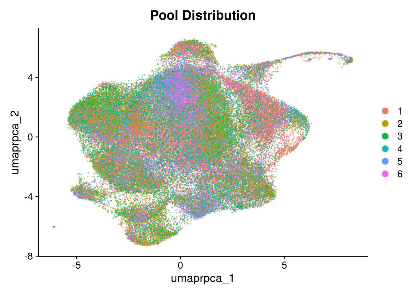
print(p5.5); print(p6); print(p6.5); print(p3.5)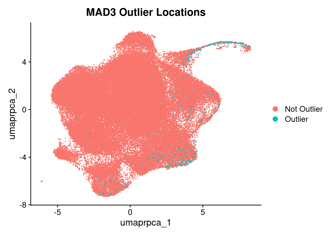
ggsave(filename = file.path(graphs_dir, int_method, cluster_resolution, glue("integrated_{int_method}_clusters_{cluster_resolution}.pdf")),       plot = p1,   width = 7,  height = 5, dpi = 300, units = "in")
ggsave(filename = file.path(graphs_dir, int_method, cluster_resolution, glue("integrated_{int_method}_sample_dist_overlaid.pdf")),                plot = p2,   width = 7,  height = 5, dpi = 300, units = "in")
ggsave(filename = file.path(graphs_dir, int_method, cluster_resolution, glue("integrated_{int_method}_sample_dist_split.pdf")),                   plot = p2.5, width = 7,  height = 5, dpi = 300, units = "in")
ggsave(filename = file.path(graphs_dir, int_method, cluster_resolution, glue("integrated_{int_method}_batch_dist.pdf")),                          plot = p3,   width = 7,  height = 5, dpi = 300, units = "in")
ggsave(filename = file.path(graphs_dir, int_method, cluster_resolution, glue("integrated_{int_method}_batch_dist_split.pdf")),                    plot = p3.5, width = 10, height = 5, dpi = 300, units = "in")
ggsave(filename = file.path(graphs_dir, int_method, cluster_resolution, glue("integrated_{int_method}_qc.pdf")),                                  plot = p4,   width = 7,  height = 5, dpi = 300, units = "in")
ggsave(filename = file.path(graphs_dir, int_method, cluster_resolution, glue("integrated_{int_method}_doublet_dist.pdf")),                        plot = p5,   width = 7,  height = 5, dpi = 300, units = "in")
ggsave(filename = file.path(graphs_dir, int_method, cluster_resolution, glue("integrated_{int_method}_outlier_dist.pdf")),                        plot = p5.5, width = 7,  height = 5, dpi = 300, units = "in")
ggsave(filename = file.path(graphs_dir, int_method, cluster_resolution, glue("integrated_{int_method}_condition_dist_overlaid.pdf")),              plot = p6,   width = 7,  height = 5, dpi = 300, units = "in")
ggsave(filename = file.path(graphs_dir, int_method, cluster_resolution, glue("integrated_{int_method}_condition_dist_split.pdf")), plot = p6.5, width = 7, height = 5, dpi = 300, units = "in")JoinLayers collapses the separate per-pool raw count matrices into a single layer, required for downstream functions. Log-normalisation corrects for differences in sequencing depth, and ScaleData z-scores expression so that highly expressed genes do not dominate dotplots and heatmaps.
DefaultAssay(merged_obj) <- "RNA"
merged_obj <- JoinLayers(merged_obj, assay = "RNA")
merged_obj <- NormalizeData(merged_obj)
merged_obj <- ScaleData(merged_obj)Module scores are calculated for all Mancuso microglial states and non-microglial cell types on the integrated object. Gene sets are re-intersected here against the merged object feature space. Scores are plotted per cluster to confirm that annotations from Part 1 hold on the clean dataset.
myeloid_seu    <- intersect(gs_myeloid,       rownames(merged_obj))
prolif_seu     <- intersect(gs_proliferating, rownames(merged_obj))
macrophage_seu <- intersect(gs_macrophage,    rownames(merged_obj))
dendritic_seu  <- intersect(gs_dendritic,     rownames(merged_obj))

gene_sets <- list(
  dendritic     = dendritic_seu,
  proliferating = prolif_seu,
  macrophage    = macrophage_seu,
  myeloid       = myeloid_seu,
  CRM           = gs_crm,
  DAM           = gs_dam,
  HLA           = gs_hla,
  HM            = gs_hm,
  IRM           = gs_irm,
  RM            = gs_rm,
  tCRM          = gs_tcrm
)

merged_obj <- AddModuleScore(merged_obj, features = gene_sets, name = names(gene_sets))

merged_obj$seurat_clusters <- factor(
  merged_obj$rpca_clusters,
  levels = sort(as.numeric(unique(as.character(merged_obj$rpca_clusters))))
)
merged_obj$seurat_clusters <- Idents(merged_obj)

p  <- VlnPlot(merged_obj, features = c("dendritic1", "proliferating2", "macrophage3", "myeloid4"),
              group.by = "seurat_clusters", pt.size = 0, ncol = 2)
p2 <- VlnPlot(merged_obj, features = c("CRM5", "DAM6", "HLA7", "HM8", "IRM9", "RM10", "tCRM11"),
              group.by = "seurat_clusters", pt.size = 0, ncol = 4)
p3 <- VlnPlot(merged_obj, features = c("nFeature_RNA"),
              group.by = "seurat_clusters", pt.size = 0, ncol = 2)

ggsave(filename = file.path(graphs_dir, int_method, cluster_resolution, glue("integrated_{int_method}_clusters_vs_nonmicroglia_{cluster_resolution}.pdf")), plot = p,  width = 7,  height = 5, dpi = 300, units = "in")
ggsave(filename = file.path(graphs_dir, int_method, cluster_resolution, glue("integrated_{int_method}_clusters_vs_mancuso_{cluster_resolution}.pdf")),      plot = p2, width = 10, height = 5, dpi = 300, units = "in")
ggsave(filename = file.path(graphs_dir, int_method, cluster_resolution, glue("integrated_{int_method}_clusters_vs_features_{cluster_resolution}.pdf")),     plot = p3, width = 10, height = 5, dpi = 300, units = "in")

print(p); print(p2); print(p3)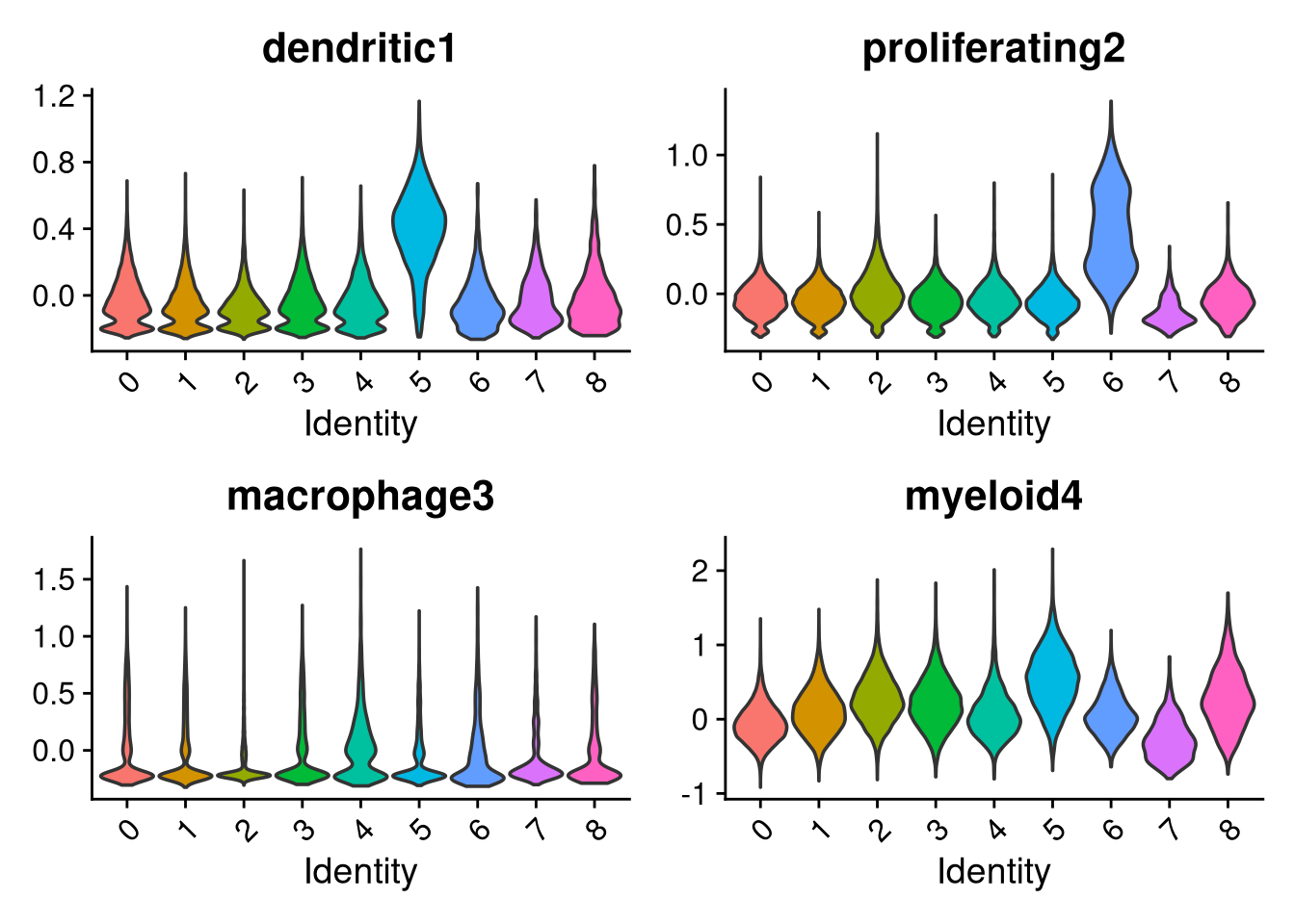
table(merged_obj$seurat_clusters)
    0     1     2     3     4     5     6     7     8
23440 16318 10089 9160 5708 4458 1905 1871 918 Marker genes are identified per cluster using a Wilcoxon rank-sum test. Only positive markers are returned, filtered to a minimum 25% detection rate and log2FC ≥ 0.25. The top 10 markers per cluster by log2FC are printed.
DefaultAssay(merged_obj) <- "RNA"
Idents(merged_obj) <- glue("{int_method}_clusters")
markers <- FindAllMarkers(
  merged_obj,
  test.use        = "wilcox",
  only.pos        = TRUE,
  min.pct         = 0.25,
  logfc.threshold = 0.25
)

write.csv(markers, file.path(objects_dir, glue("wilcox_markers_{cluster_resolution}.csv")))

top10_markers <- markers %>%
  group_by(cluster) %>%
  slice_max(n = 10, order_by = avg_log2FC)

top10_markersp <- VlnPlot(merged_obj, features = "percent.mt", pt.size = 0) +
geom_hline(yintercept = 15, linetype = "dashed", color = "red")
ggsave(
filename = file.path(graphs_dir, int_method, cluster_resolution, glue("integrated_{int_method}_clusters_vs_mt_{cluster_resolution}.pdf")),
plot = p, width = 10, height = 5, dpi = 300, units = "in"
)Warning: Removed 1 row containing missing values or values outside the scale range
(`geom_hline()`).Cluster labels are assigned based on Mancuso microglial state signatures and top marker genes identified in the previous section. Labels are applied to the Seurat identity slot for downstream plotting.
new_cluster_ids <- c(
  "0" = "HM_1",
  "1" = "tCRM_1",
  "2" = "DAM/HLA",
  "3" = "tCRM_2",
  "4" = "IRM",
  "5" = "HLA/myeloid",
  "6" = "Proliferating",
  "7" = "HM_2",
  "8" = "CRM"
)

merged_obj <- RenameIdents(merged_obj, new_cluster_ids)

p <- DimPlot(merged_obj, reduction = "umap.rpca", label = TRUE, repel = TRUE)
print(p)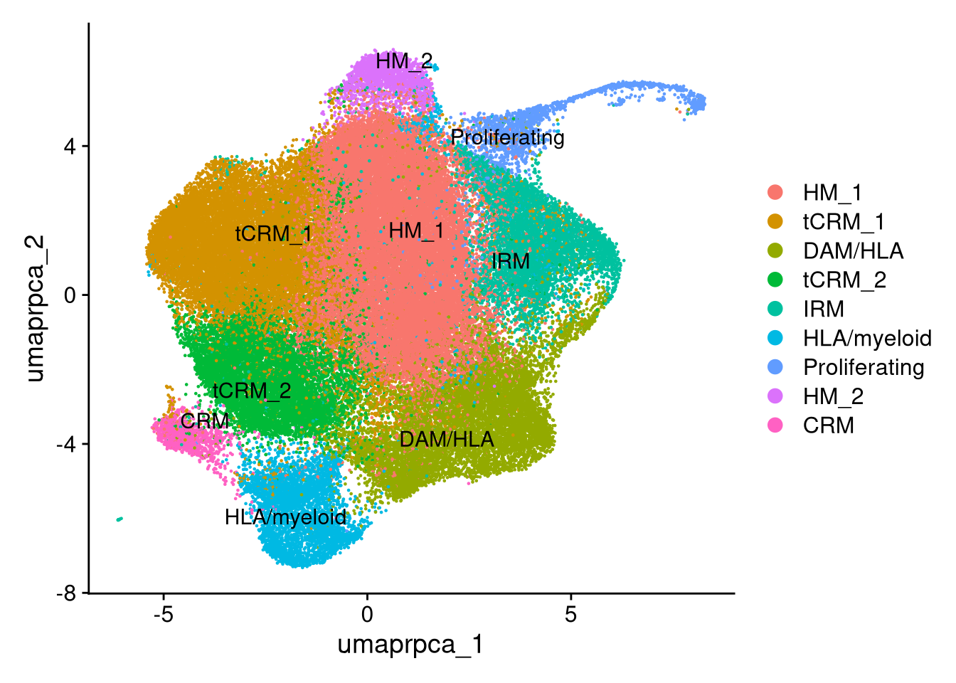
ggsave(
  filename = file.path(graphs_dir, int_method, cluster_resolution, glue("labelled_integrated_{cluster_resolution}.png")),
  plot = p,
  device = ragg::agg_png,
  width = 7, height = 5, dpi = 300, units = "in"
)qs_save(merged_obj, file.path(objects_dir, glue("labelled_integrated_{cluster_resolution}.qs2")))The standard DimPlot output is refined with custom L-shaped axis arrows, bold halo labels positioned at cluster centroids, and a total cell count annotation. This produces a publication-ready version of the labelled embedding.
cluster_counts <- table(Idents(merged_obj))
new_labels     <- paste0(names(cluster_counts), "\n n = ", comma(as.numeric(cluster_counts)))
names(new_labels) <- names(cluster_counts)
merged_obj_plot   <- RenameIdents(merged_obj, new_labels)

umap_coords         <- data.frame(Embeddings(merged_obj_plot, "umap.rpca"))
umap_coords$cluster <- Idents(merged_obj_plot)
centroids           <- aggregate(cbind(umaprpca_1, umaprpca_2) ~ cluster, data = umap_coords, mean)

x_range <- range(umap_coords[, 1])
y_range <- range(umap_coords[, 2])

axis_origin_x <- x_range[1] - (diff(x_range) * 0.1)
axis_origin_y <- y_range[1] - (diff(y_range) * 0.1)
axis_length   <- diff(x_range) * 0.2

p <- DimPlot(merged_obj_plot,
             reduction = "umap.rpca",
             label     = FALSE,
             pt.size   = 0.1) +
  NoLegend() +
  NoAxes() +
  theme(plot.title = element_blank()) +
  geom_text_repel(data = centroids,
                  aes(x = umaprpca_1, y = umaprpca_2, label = cluster),
                  fontface          = "bold",
                  size              = 4.5,
                  color             = "black",
                  bg.color          = "white",
                  bg.r              = 0.15,
                  force             = 5,
                  min.segment.length = 0) +
  annotate("segment",
           x = axis_origin_x, xend = axis_origin_x + axis_length,
           y = axis_origin_y, yend = axis_origin_y,
           arrow = arrow(length = unit(0.2, "cm"), type = "closed"),
           size = 1.2, lineend = "round") +
  annotate("segment",
           x = axis_origin_x, xend = axis_origin_x,
           y = axis_origin_y, yend = axis_origin_y + axis_length,
           arrow = arrow(length = unit(0.2, "cm"), type = "closed"),
           size = 1.2, lineend = "round") +
  annotate("text",
           x = axis_origin_x + (axis_length / 2), y = axis_origin_y - 1,
           label = "UMAP 1", hjust = 0.5, vjust = 1, fontface = "bold") +
  annotate("text",
           x = axis_origin_x - 1, y = axis_origin_y + (axis_length / 2),
           label = "UMAP 2", angle = 90, hjust = 1, vjust = 0.5, fontface = "bold") +
  annotate("text",
           x = mean(x_range), y = axis_origin_y - 2.5,
           label = paste0("Total cells = ", comma(length(Cells(merged_obj)))),
           size = 5, fontface = "bold")
Warning: Using `size` aesthetic for lines was deprecated in ggplot2 3.4.0.
ℹ Please use `linewidth` instead.print(p)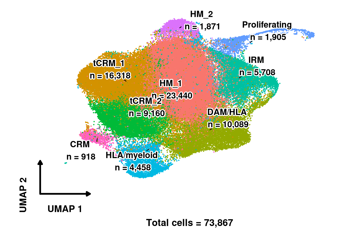
ggsave(
  filename = file.path(graphs_dir, int_method, cluster_resolution, glue("labelled_polished_{cluster_resolution}.pdf")),
  plot     = p,
  device   = cairo_pdf,
  width = 8, height = 6, dpi = 300, units = "in"
)sessionInfo()R version 4.5.1 (2025-06-13)
Platform: x86_64-pc-linux-gnu
Running under: Rocky Linux 8.7 (Green Obsidian)
Matrix products: default
BLAS/LAPACK: FlexiBLAS OPENBLAS; LAPACK version 3.12.0
locale:
[1] LC_CTYPE=en_GB.UTF-8 LC_NUMERIC=C
[3] LC_TIME=en_GB.UTF-8 LC_COLLATE=en_GB.UTF-8
[5] LC_MONETARY=en_GB.UTF-8 LC_MESSAGES=en_GB.UTF-8
[7] LC_PAPER=en_GB.UTF-8 LC_NAME=C
[9] LC_ADDRESS=C LC_TELEPHONE=C
[11] LC_MEASUREMENT=en_GB.UTF-8 LC_IDENTIFICATION=C
time zone: Europe/London
tzcode source: system (glibc)
attached base packages:
[1] stats4 stats graphics grDevices utils datasets methods
[8] base
other attached packages:
[1] ggrepel_0.9.6 scales_1.4.0
[3] presto_1.0.0 data.table_1.18.2.1
[5] Rcpp_1.1.1 qs2_0.1.6
[7] scDblFinder_1.24.10 SingleCellExperiment_1.32.0
[9] SummarizedExperiment_1.40.0 Biobase_2.70.0
[11] GenomicRanges_1.62.1 Seqinfo_1.0.0
[13] IRanges_2.44.0 S4Vectors_0.48.0
[15] BiocGenerics_0.56.0 generics_0.1.4
[17] MatrixGenerics_1.22.0 matrixStats_1.5.0
[19] SoupX_1.6.2 gridExtra_2.3
[21] future_1.70.0 readxl_1.4.5
[23] glue_1.8.0 lubridate_1.9.4
[25] forcats_1.0.1 stringr_1.6.0
[27] purrr_1.2.1 readr_2.1.6
[29] tidyr_1.3.2 tibble_3.3.1
[31] ggplot2_4.0.2 tidyverse_2.0.0
[33] Seurat_5.3.1.9001 SeuratObject_5.3.0.9003
[35] sp_2.2-1 Matrix_1.7-4
[37] dplyr_1.2.0
loaded via a namespace (and not attached):
[1] RcppAnnoy_0.0.23 splines_4.5.1
[3] later_1.4.6 BiocIO_1.20.0
[5] bitops_1.0-9 cellranger_1.1.0
[7] polyclip_1.10-7 XML_3.99-0.20
[9] fastDummies_1.7.5 lifecycle_1.0.5
[11] edgeR_4.8.1 globals_0.19.1
[13] lattice_0.22-7 MASS_7.3-65
[15] magrittr_2.0.4 limma_3.66.0
[17] plotly_4.12.0 rmarkdown_2.30
[19] yaml_2.3.12 metapod_1.18.0
[21] httpuv_1.6.16 otel_0.2.0
[23] glmGamPoi_1.22.0 sctransform_0.4.3
[25] spam_2.11-3 spatstat.sparse_3.1-0
[27] reticulate_1.45.0 cowplot_1.2.0
[29] pbapply_1.7-4 RColorBrewer_1.1-3
[31] abind_1.4-8 Rtsne_0.17
[33] RCurl_1.98-1.17 irlba_2.3.7
[35] listenv_0.10.1 spatstat.utils_3.2-1
[37] goftest_1.2-3 RSpectra_0.16-2
[39] dqrng_0.4.1 spatstat.random_3.4-4
[41] fitdistrplus_1.2-6 parallelly_1.46.1
[43] DelayedMatrixStats_1.32.0 codetools_0.2-20
[45] DelayedArray_0.36.0 scuttle_1.20.0
[47] tidyselect_1.2.1 UCSC.utils_1.6.1
[49] farver_2.1.2 viridis_0.6.5
[51] ScaledMatrix_1.18.0 spatstat.explore_3.7-0
[53] GenomicAlignments_1.46.0 jsonlite_2.0.0
[55] BiocNeighbors_2.4.0 progressr_0.19.0
[57] scater_1.38.0 ggridges_0.5.7
[59] survival_3.8-3 systemfonts_1.3.1
[61] tools_4.5.1 ragg_1.5.0
[63] ica_1.0-3 SparseArray_1.10.8
[65] xfun_0.56 GenomeInfoDb_1.46.2
[67] withr_3.0.2 fastmap_1.2.0
[69] bluster_1.20.0 digest_0.6.39
[71] rsvd_1.0.5 timechange_0.3.0
[73] R6_2.6.1 mime_0.13
[75] textshaping_1.0.3 scattermore_1.2
[77] tensor_1.5.1 spatstat.data_3.1-9
[79] cigarillo_1.0.0 rtracklayer_1.70.0
[81] httr_1.4.8 htmlwidgets_1.6.4
[83] S4Arrays_1.10.1 uwot_0.2.4
[85] pkgconfig_2.0.3 gtable_0.3.6
[87] lmtest_0.9-40 S7_0.2.1
[89] XVector_0.50.0 htmltools_0.5.9
[91] dotCall64_1.2 png_0.1-8
[93] spatstat.univar_3.1-6 scran_1.38.0
[95] knitr_1.51 tzdb_0.5.0
[97] reshape2_1.4.5 rjson_0.2.23
[99] nlme_3.1-168 curl_7.0.0
[101] zoo_1.8-15 KernSmooth_2.23-26
[103] vipor_0.4.7 parallel_4.5.1
[105] miniUI_0.1.2 ggrastr_1.0.2
[107] restfulr_0.0.16 pillar_1.11.1
[109] grid_4.5.1 vctrs_0.7.1
[111] RANN_2.6.2 promises_1.5.0
[113] stringfish_0.17.0 BiocSingular_1.26.1
[115] beachmat_2.26.0 xtable_1.8-4
[117] cluster_2.1.8.1 beeswarm_0.4.0
[119] evaluate_1.0.5 locfit_1.5-9.12
[121] cli_3.6.5 compiler_4.5.1
[123] Rsamtools_2.26.0 rlang_1.1.7
[125] crayon_1.5.3 future.apply_1.20.2
[127] labeling_0.4.3 ggbeeswarm_0.7.3
[129] plyr_1.8.9 stringi_1.8.7
[131] viridisLite_0.4.3 deldir_2.0-4
[133] BiocParallel_1.44.0 Biostrings_2.78.0
[135] lazyeval_0.2.2 spatstat.geom_3.7-0
[137] RcppHNSW_0.6.0 hms_1.1.4
[139] patchwork_1.3.2 sparseMatrixStats_1.22.0
[141] statmod_1.5.1 shiny_1.12.1
[143] ROCR_1.0-12 igraph_2.2.2
[145] RcppParallel_5.1.11-1 xgboost_3.2.0.1