glmmTMB DE (volcanos)

Visualises differential expression results from the glmmTMB model fitted in scripts/glmmTMB.qmd. Produces an interaction logFC scatter plot, per-gene violin and pseudobulk boxplots, eCDF plots, and ISG/top-gene summaries.

Inputs: output/run1/objects/glmmTMB_with_interactions_corrected.qs2, output/run1/objects/prelabelled_integrated_rpca.qs2 Outputs: PDF figures written to output/run1/graphs/

Load libraries

Code

library(Seurat)
library(glmmTMB)
library(qs2)
library(dplyr)
library(tidyr)
library(ggplot2)
library(ggrepel)

Load directories

Code

run_num <- "run1"


out_dir <- file.path("output", run_num)
graphs_dir <- file.path(out_dir, "graphs")
objects_dir <- file.path(out_dir, "objects")

dir.create(graphs_dir, recursive = TRUE, showWarnings = FALSE)
dir.create(objects_dir, recursive = TRUE, showWarnings = FALSE)

Load data

Code

required_inputs <- c(
  file.path(objects_dir, "glmmTMB_with_interactions_corrected.qs2"),
  file.path(objects_dir, "prelabelled_integrated_rpca.qs2")
)
missing <- required_inputs[!file.exists(required_inputs)]
if (length(missing) > 0) {
  message("Required inputs not found:\n", paste(" -", missing, collapse = "\n"),
          "\nRun scripts/glmmTMB.qmd and seurat_trisomy_v1/v2.qmd first.")
  knitr::knit_exit()
}
final_df <- qs_read(required_inputs[1])

seurat_obj <- qs_read(required_inputs[2])

Interaction scatter plot

Code

plot_data <- final_df %>%
  # 1. Keep only the rows where we are looking at the Ploidy effect (A vs B)
  # and ensure Background is one of our two target groups.
  filter(contrast == "A - B", !is.na(Background)) %>% 
  
  # 2. Select only the necessary columns. 
  # Important: Interaction_FDR must be the same for both rows of a gene 
  # or you'll get duplicates again.
  select(Gene, Background, estimate, Interaction_FDR) %>%
  
  # 3. Pivot: this should now have 1 row per Gene
  pivot_wider(names_from = Background, values_from = estimate) %>%
  
  # 4. Create labeling logic
  mutate(
    Significance = ifelse(Interaction_FDR < 0.05, "Significant Interaction", "Not Significant"),
    Label = ifelse(Interaction_FDR < 0.05, Gene, NA)
  )

Code

p <- ggplot(plot_data, aes(x = NLGF, y = hAPP)) +
  # Draw the non-significant genes first so they fall in the background
  geom_point(data = filter(plot_data, Significance == "Not Significant"), 
             color = "grey80", alpha = 0.5, size = 1.5) +
  
  # Draw your 23 significant genes on top in a bold color
  geom_point(data = filter(plot_data, Significance == "Significant Interaction"), 
             color = "red", alpha = 0.9, size = 2.5) +
  
  # Add the "Zero" crosshairs to divide it into quadrants
  geom_hline(yintercept = 0, linetype = "dotted", color = "black") +
  geom_vline(xintercept = 0, linetype = "dotted", color = "black") +
  
  # Add the diagonal "Line of No Interaction" (Slope = 1, Intercept = 0)
  geom_abline(intercept = 0, slope = 1, linetype = "dashed", color = "darkblue", linewidth = 0.8) +
  
  # Add the repelling text labels for the 23 genes
  geom_text_repel(aes(label = Label), 
                  color = "black", 
                  size = 4, 
                  fontface = "bold",
                  box.padding = 0.5, 
                  max.overlaps = Inf) + # Ensures it tries to plot all 23 labels
  
  # Aesthetics
  theme_minimal() +
  labs(
    title = "Interaction Landscape: Trisomy Effect by Plaque Background",
    x = "Log2 Fold Change (Trisomic vs Disomic in NLGF)",
    y = "Log2 Fold Change (Trisomic vs Disomic in hAPP)"
  ) +
  theme(
    plot.title = element_text(face = "bold", size = 14),
    axis.title = element_text(face = "bold")
  )

print(p)

Warning: Removed 14629 rows containing missing values or values outside the scale range
(`geom_text_repel()`).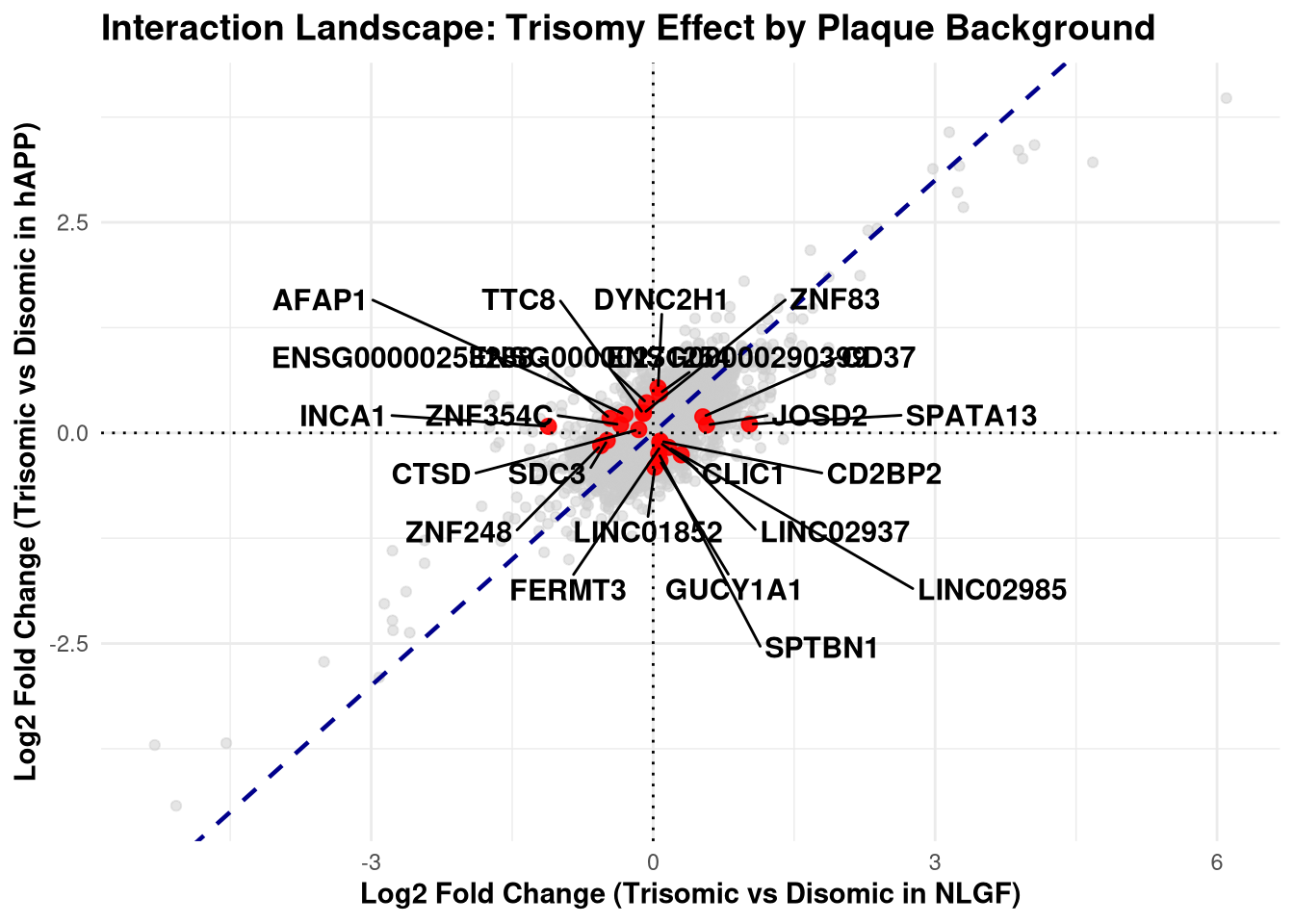

Code

ggsave(
  file.path(graphs_dir, "interaction_logFC_scatterplot.pdf"), 
  plot = p, 
  width = 12, 
  height = 6, 
  units = "in"
  )

Warning: Removed 14629 rows containing missing values or values outside the scale range
(`geom_text_repel()`).

Per-gene violin plots

Code

#Extract signficant interaction genes from plot data
sig_genes <- plot_data %>%
  filter(Significance == "Significant Interaction") %>%
  pull(Gene)
sig_genes

 [1] "AFAP1"           "CD2BP2"          "CD37"            "CLIC1"          
 [5] "CTSD"            "DYNC2H1"         "ENSG00000253288" "ENSG00000271254"
 [9] "ENSG00000290399" "FERMT3"          "GUCY1A1"         "INCA1"          
[13] "JOSD2"           "LINC01852"       "LINC02937"       "LINC02985"      
[17] "SDC3"            "SPATA13"         "SPTBN1"          "TTC8"           
[21] "ZNF248"          "ZNF354C"         "ZNF83"

Code

#Pull raw counts for these genes
expr_matrix <- GetAssayData(seurat_obj, assay = "SCT", layer = "data")[sig_genes, ]
expr_df <- as.data.frame(t(as.matrix(expr_matrix)))
expr_df$CellID <- rownames(expr_df)
expr_df$Ploidy <- factor(seurat_obj@meta.data$microglia, levels = c("B", "A"))
expr_df$Background <- factor(seurat_obj@meta.data$app_genotype, levels = c("NLGF", "hAPP"))
expr_df$Mouse <- seurat_obj@meta.data$orig.ident
expr_df$Condition <- factor(seurat_obj@meta.data$group_id)

# Pivot to "Long" format for ggplot2
expr_long <- expr_df %>%
  pivot_longer(cols = any_of(sig_genes), names_to = "Gene", values_to = "Expression")

pdf_file <- file.path(graphs_dir, "Interaction_Genes_Raw_Violins.pdf")
pdf(pdf_file, width = 8, height = 6)

for (gene in sig_genes) {
  
  # Filter data for the current gene
  gene_data <- expr_long %>% filter(Gene == gene)
  
  # Create the plot
  p <- ggplot(gene_data, aes(x = Condition, y = Expression, fill = Background)) +
    # scale="width" ensures all violins are the same width regardless of cell count
    geom_violin(scale = "width", alpha = 0.7, color = "black") + 
    
    # Add a point for the mean expression to help guide the eye
    stat_summary(fun = mean, geom = "point", shape = 23, size = 3, fill = "white") +
    
    scale_fill_manual(values = c("NLGF" = "#4C72B0", "hAPP" = "#C44E52")) +
    theme_minimal(base_size = 14) +
    labs(
      title = paste("Expression of", gene),
      subtitle = "Significant Ploidy * Background Interaction",
      x = "Condition",
      y = "Raw Counts"
    ) +
    theme(
      plot.title = element_text(face = "bold", hjust = 0.5),
      plot.subtitle = element_text(hjust = 0.5),
      axis.text.x = element_text(face = "bold"),
      legend.position = "none" # We don't need a legend since the X-axis is labeled
    )
  
  print(p) # Print each plot as a new page in the PDF
}

dev.off() # Close and save the PDF

png 
  2

Code

cat("Saved 23 violin plots to:", pdf_file, "\n")

Saved 23 violin plots to: output/run1/graphs/Interaction_Genes_Raw_Violins.pdf

Dotplot

Code

p_dot <- DotPlot(seurat_obj, 
                 features = sig_genes, 
                 group.by = "group_id",
                 assay = "SCT") +
  
  # Improve the aesthetics for a large number of genes
  theme(axis.text.x = element_text(angle = 45, hjust = 1, face = "bold.italic"),
        axis.text.y = element_text(face = "bold", size = 12),
        plot.title = element_text(face = "bold", hjust = 0.5)) +
  
  # Custom colors: Low expression is light grey, high expression is dark red
  scale_color_gradient(low = "lightgrey", high = "#C44E52") +
  
  labs(title = "Significant Ploidy * Background Interaction Genes",
       x = "Gene",
       y = "Condition")

Warning: Scaling data with a low number of groups may produce misleading
results

Scale for colour is already present.
Adding another scale for colour, which will replace the existing scale.

Code

# 3. SAVE TO PDF
# Because you have 23 genes, a wider PDF (e.g., width = 12) prevents the gene names from squishing
dp_file <- file.path(graphs_dir, "Interaction_Genes_DotPlot.pdf")
pdf(dp_file, width = 12, height = 5)
print(p_dot)
dev.off()

png 
  2

Code

cat("DotPlot saved to:", dp_file, "\n")

DotPlot saved to: output/run1/graphs/Interaction_Genes_DotPlot.pdf

Pseudobulk count plots

Code

# Collapse the single cells down to one average value per mouse
pb_long <- expr_long %>%
  # We group by Mouse, Condition, and Background so we keep those labels for plotting
  group_by(Mouse, Condition, Background, Gene) %>%
  summarise(Pseudobulk_Expression = mean(Expression), .groups = "drop")

# 4. PLOT AND SAVE TO PDF
pdf_file <- file.path(graphs_dir, "Interaction_Genes_Pseudobulk.pdf")
pdf(pdf_file, width = 8, height = 6)

for (gene in sig_genes) {
  
  # Filter data for the current gene
  gene_pb <- pb_long %>% filter(Gene == gene)
  
  # Create the boxplot
  p <- ggplot(gene_pb, aes(x = Condition, y = Pseudobulk_Expression, fill = Background)) +
    
    # Add the boxplot structure (hide outliers since we will draw all mice manually)
    geom_boxplot(alpha = 0.5, outlier.shape = NA) +
    
    # Draw every single mouse as a distinct dot (jittered slightly so they don't overlap)
    geom_jitter(width = 0.2, size = 3, shape = 21, color = "black", stroke = 1) +
    
    # Use your defined colors for the background
    scale_fill_manual(values = c("NLGF" = "#4C72B0", "hAPP" = "#C44E52")) +
    
    theme_minimal(base_size = 14) +
    labs(
      title = paste(gene, "- Pseudobulk Expression"),
      subtitle = "Each dot represents the average normalized expression of one mouse",
      x = "Condition",
      y = "Mean SCT Normalized Expression"
    ) +
    theme(
      plot.title = element_text(face = "bold", hjust = 0.5),
      plot.subtitle = element_text(hjust = 0.5),
      # Angle the X-axis labels in case your group_id names are long
      axis.text.x = element_text(face = "bold", angle = 45, hjust = 1),
      legend.position = "none" # Hide legend since X-axis/colors explain it
    )
  
  print(p) # Print each plot as a new page in the PDF
}

dev.off() # Close and save the PDF

png 
  2

Code

cat("Saved pseudobulked boxplots to:", pdf_file, "\n")

Saved pseudobulked boxplots to: output/run1/graphs/Interaction_Genes_Pseudobulk.pdf

ECDF (non-zero cells)

Code

ecdf_pdf_file <- file.path(graphs_dir, "Interaction_Genes_NonZero_eCDF_with_Proportions.pdf")
pdf(ecdf_pdf_file, width = 10, height = 7)

for (gene in sig_genes) {
  
  # 1. Get data for the specific gene
  gene_data_all <- expr_long %>% filter(Gene == gene)
  
  # 2. Calculate the proportion of non-zero cells per group
  stats_summary <- gene_data_all %>%
    group_by(Condition) %>%
    summarise(
      total_cells = n(),
      non_zero_cells = sum(Expression > 0),
      prop_expressing = (non_zero_cells / total_cells) * 100,
      .groups = "drop"
    ) %>%
    mutate(label = paste0(Condition, ": ", round(prop_expressing, 1), "%"))

  # Create a string to display as a subtitle
  prop_text <- paste("Expressing Cells % -", paste(stats_summary$label, collapse = " | "))
  
  # 3. Filter for non-zero cells for the eCDF
  gene_data_nonzero <- gene_data_all %>% filter(Expression > 0)
  
  if(nrow(gene_data_nonzero) < 5) {
    message("Skipping ", gene, " - too few expressing cells.")
    next
  }
  
  # 4. Create the plot
  p_ecdf <- ggplot(gene_data_nonzero, aes(x = Expression, color = Condition)) +
    stat_ecdf(geom = "step", linewidth = 1.2) +
    # We use a log scale if the data is highly skewed, but SCT is usually okay on linear
    theme_minimal(base_size = 12) +
    labs(
      title = paste(gene, "- Non-Zero Distribution"),
      subtitle = prop_text,
      x = "SCT Normalized Expression (Non-Zero Only)",
      y = "Cumulative Fraction of Expressing Cells",
      color = "Condition"
    ) +
    theme(
      plot.title = element_text(face = "bold", size = 16),
      plot.subtitle = element_text(size = 9, color = "blue4"),
      legend.position = "bottom",
      panel.grid.minor = element_blank()
    )
  
  print(p_ecdf)
}

dev.off()

png 
  2

Code

cat("Saved annotated eCDF plots to:", ecdf_pdf_file, "\n")

Saved annotated eCDF plots to: output/run1/graphs/Interaction_Genes_NonZero_eCDF_with_Proportions.pdf

ECDF (all cells)

Code

# Updated file name to reflect all cells
ecdf_pdf_file <- file.path(graphs_dir, "Interaction_Genes_AllCells_eCDF_with_Proportions.pdf")
pdf(ecdf_pdf_file, width = 10, height = 7)

for (gene in sig_genes) {
  
  # 1. Get data for the specific gene (includes all zeros)
  gene_data_all <- expr_long %>% filter(Gene == gene)
  
  # 2. Calculate the proportion of non-zero cells per group
  stats_summary <- gene_data_all %>%
    group_by(Condition) %>%
    summarise(
      total_cells = n(),
      non_zero_cells = sum(Expression > 0),
      prop_expressing = (non_zero_cells / total_cells) * 100,
      .groups = "drop"
    ) %>%
    mutate(label = paste0(Condition, ": ", round(prop_expressing, 1), "%"))

  # Create a string to display as a subtitle
  prop_text <- paste("Expressing Cells % -", paste(stats_summary$label, collapse = " | "))
  
  # 3. Check to ensure we have enough total cells to plot
  if(nrow(gene_data_all) < 5) {
    message("Skipping ", gene, " - too few total cells.")
    next
  }
  
  # 4. Create the plot using gene_data_all instead of gene_data_nonzero
  p_ecdf <- ggplot(gene_data_all, aes(x = Expression, color = Condition)) +
    stat_ecdf(geom = "step", linewidth = 1.2) +
    theme_minimal(base_size = 12) +
    labs(
      title = paste(gene, "- All Cells Distribution"),
      subtitle = prop_text,
      x = "SCT Normalized Expression (All Cells)",
      y = "Cumulative Fraction of Total Cells",
      color = "Condition"
    ) +
    theme(
      plot.title = element_text(face = "bold", size = 16),
      plot.subtitle = element_text(size = 9, color = "blue4"),
      legend.position = "bottom",
      panel.grid.minor = element_blank()
    )
  
  print(p_ecdf)
}

dev.off()

png 
  2

Code

cat("Saved annotated eCDF plots to:", ecdf_pdf_file, "\n")

Saved annotated eCDF plots to: output/run1/graphs/Interaction_Genes_AllCells_eCDF_with_Proportions.pdf

ISG gene pseudobulk plots

Code

isg_genes <- c("IFI27", "IFI44L", "IFIT1", "IFIT2", "IFIT3", 
               "MX1", "MX2", "OAS1", "ISG15", "USP18", 
               "RSAD2", "LY6E", "DDX60", "TRIM25", "STAT1", "IRF7")

isg_nlgf <- final_df %>%
  filter(Background == "NLGF" & contrast == "A - B") %>% 
  arrange(FDR) %>% 
  filter(Gene %in% isg_genes) %>%
  slice_head(n = 10) 

isg_happ <- final_df %>%
  filter(Background == "hAPP" & contrast == "A - B") %>% 
  arrange(FDR) %>% 
  filter(Gene %in% isg_genes) %>%
  slice_head(n = 10) 

expr_matrix <- GetAssayData(seurat_obj, assay = "SCT", layer = "data")[isg_genes, ]
expr_df <- as.data.frame(t(as.matrix(expr_matrix)))
expr_df$CellID <- rownames(expr_df)
expr_df$Ploidy <- factor(seurat_obj@meta.data$microglia, levels = c("B", "A"))
expr_df$Background <- factor(seurat_obj@meta.data$app_genotype, levels = c("NLGF", "hAPP"))
expr_df$Mouse <- seurat_obj@meta.data$orig.ident
expr_df$Condition <- factor(seurat_obj@meta.data$group_id)

expr_long <- expr_df %>%
  pivot_longer(cols = any_of(isg_genes), names_to = "Gene", values_to = "Expression")


# Collapse the single cells down to one average value per mouse
pb_long <- expr_long %>%
  # We group by Mouse, Condition, and Background so we keep those labels for plotting
  group_by(Mouse, Condition, Background, Gene) %>%
  summarise(Pseudobulk_Expression = mean(Expression), .groups = "drop") 
# 4. PLOT AND SAVE TO PDF
pdf_file <- file.path(graphs_dir, "ISG_genes_Pseudobulk_glmmtmb.pdf")
pdf(pdf_file, width = 8, height = 6)

for (gene in isg_genes) {
  
  # Filter data for the current gene
  gene_pb <- pb_long %>% filter(Gene == gene)
  
  # Extract the FDR values for BOTH backgrounds from final_df
  nlgf_fdr_raw <- final_df %>% filter(Gene == gene & Background == "NLGF" & contrast == "A - B") %>% pull(FDR)
  happ_fdr_raw <- final_df %>% filter(Gene == gene & Background == "hAPP" & contrast == "A - B") %>% pull(FDR)
  
  # Format cleanly, handling potential missing values gracefully
  fmt_nlgf <- ifelse(length(nlgf_fdr_raw) > 0, signif(nlgf_fdr_raw, digits = 3), "N/A")
  fmt_happ <- ifelse(length(happ_fdr_raw) > 0, signif(happ_fdr_raw, digits = 3), "N/A")
  
  
  # Create the boxplot
  p <- ggplot(gene_pb, aes(x = Condition, y = Pseudobulk_Expression, fill = Background)) +
    
    # Add the boxplot structure (hide outliers since we will draw all mice manually)
    geom_boxplot(alpha = 0.5, outlier.shape = NA) +
    
    # Draw every single mouse as a distinct dot (jittered slightly so they don't overlap)
    geom_jitter(width = 0.2, size = 3, shape = 21, color = "black", stroke = 1) +
    
    # Use your defined colors for the background
    scale_fill_manual(values = c("NLGF" = "#4C72B0", "hAPP" = "#C44E52")) +
    
    theme_minimal(base_size = 14) +
    labs(
      title = paste(gene, "- Pseudobulk Expression"),
      subtitle = paste0("FDR (NLGF): ", fmt_nlgf, "  |  FDR (hAPP): ", fmt_happ, "\nEach dot = average expression of one mouse"),
      x = "Condition",
      y = "Mean SCT Normalized Expression"
    ) +
    theme(
      plot.title = element_text(face = "bold", hjust = 0.5),
      plot.subtitle = element_text(hjust = 0.5),
      # Angle the X-axis labels in case your group_id names are long
      axis.text.x = element_text(face = "bold", angle = 45, hjust = 1),
      legend.position = "none" # Hide legend since X-axis/colors explain it
    )
  
  print(p) # Print each plot as a new page in the PDF
}

dev.off() # Close and save the PDF

png 
  2

Code

cat("Saved pseudobulked boxplots to:", pdf_file, "\n")

Saved pseudobulked boxplots to: output/run1/graphs/ISG_genes_Pseudobulk_glmmtmb.pdf

Top/bottom DE genes — NLGF trisomy effect

Code

pb_long <- expr_long %>%
  # We group by Mouse, Condition, and Background so we keep those labels for plotting
  group_by(Mouse, Condition, Background, Gene) %>%
  summarise(Pseudobulk_Expression = mean(Expression), .groups = "drop")


top10_sig <- final_df %>%
  filter(Background == "NLGF" & contrast == "A - B") %>% 
  arrange(FDR) %>% 
  filter(estimate > 0) %>%
  slice_head(n = 10) 

bot10_sig <- final_df %>%
  filter(Background == "NLGF" & contrast == "A - B") %>% 
  arrange(FDR) %>% 
  filter(estimate < 0) %>%
  slice_head(n = 10) 

top_bottom_res <- bind_rows(top10_sig, bot10_sig)
target_genes <- top_bottom_res$Gene

pdf_file <- file.path(graphs_dir, "ISG_genes_top_bottom_nlgf_a_vs_b.pdf")
pdf(pdf_file, width = 8, height = 6)
for (gene in target_genes) {
  
  # Filter data for the current gene
  gene_pb <- pb_long %>% filter(Gene == gene)
  
  # Extract the FDR value for this specific gene from the glmmTMB results table
  # Using signif() to format it cleanly (e.g., 0.000123 -> 1.23e-04)
  gene_fdr <- top_bottom_res %>% filter(Gene == gene) %>% pull(FDR)
  formatted_fdr <- signif(gene_fdr, digits = 3)
  
  # Create the boxplot
  p <- ggplot(gene_pb, aes(x = Condition, y = Pseudobulk_Expression, fill = Background)) +
    
    # Add the boxplot structure (hide outliers since we will draw all mice manually)
    geom_boxplot(alpha = 0.5, outlier.shape = NA) +
    
    # Draw every single mouse as a distinct dot (jittered slightly so they don't overlap)
    geom_jitter(width = 0.2, size = 3, shape = 21, color = "black", stroke = 1) +
    
    # Use your defined colors for the background
    scale_fill_manual(values = c("NLGF" = "#4C72B0", "hAPP" = "#C44E52")) +
    
    theme_minimal(base_size = 14) +
    labs(
      title = paste(gene, "- Pseudobulk Expression"),
      subtitle = paste0("glmmTMB FDR: ", formatted_fdr, " | Each dot = average expression of one mouse"),
      x = "Condition",
      y = "Mean SCT Normalized Expression"
    ) +
    theme(
      plot.title = element_text(face = "bold", hjust = 0.5),
      plot.subtitle = element_text(hjust = 0.5),
      # Angle the X-axis labels in case your group_id names are long
      axis.text.x = element_text(face = "bold", angle = 45, hjust = 1),
      legend.position = "none" # Hide legend since X-axis/colors explain it
    )
  
  print(p) # Print each plot as a new page in the PDF
}

Warning: No shared levels found between `names(values)` of the manual scale and the
data's fill values.
No shared levels found between `names(values)` of the manual scale and the
data's fill values.
No shared levels found between `names(values)` of the manual scale and the
data's fill values.
No shared levels found between `names(values)` of the manual scale and the
data's fill values.
No shared levels found between `names(values)` of the manual scale and the
data's fill values.
No shared levels found between `names(values)` of the manual scale and the
data's fill values.
No shared levels found between `names(values)` of the manual scale and the
data's fill values.
No shared levels found between `names(values)` of the manual scale and the
data's fill values.
No shared levels found between `names(values)` of the manual scale and the
data's fill values.
No shared levels found between `names(values)` of the manual scale and the
data's fill values.
No shared levels found between `names(values)` of the manual scale and the
data's fill values.
No shared levels found between `names(values)` of the manual scale and the
data's fill values.
No shared levels found between `names(values)` of the manual scale and the
data's fill values.
No shared levels found between `names(values)` of the manual scale and the
data's fill values.
No shared levels found between `names(values)` of the manual scale and the
data's fill values.
No shared levels found between `names(values)` of the manual scale and the
data's fill values.
No shared levels found between `names(values)` of the manual scale and the
data's fill values.
No shared levels found between `names(values)` of the manual scale and the
data's fill values.
No shared levels found between `names(values)` of the manual scale and the
data's fill values.
No shared levels found between `names(values)` of the manual scale and the
data's fill values.

Code

dev.off() # Close and save the PDF

png 
  2

Code

cat("Saved pseudobulked boxplots to:", pdf_file, "\n")

Saved pseudobulked boxplots to: output/run1/graphs/ISG_genes_top_bottom_nlgf_a_vs_b.pdf

Top/bottom DE genes — hAPP trisomy effect

Code

pb_long <- expr_long %>%
  # We group by Mouse, Condition, and Background so we keep those labels for plotting
  group_by(Mouse, Condition, Background, Gene) %>%
  summarise(Pseudobulk_Expression = mean(Expression), .groups = "drop")


top10_sig <- final_df %>%
  filter(Background == "hAPP" & contrast == "A - B") %>% 
  arrange(FDR) %>% 
  filter(estimate > 0) %>%
  slice_head(n = 10) 

bot10_sig <- final_df %>%
  filter(Background == "hAPP" & contrast == "A - B") %>% 
  arrange(FDR) %>% 
  filter(estimate < 0) %>%
  slice_head(n = 10) 

top_bottom_res <- bind_rows(top10_sig, bot10_sig)
target_genes <- top_bottom_res$Gene

pdf_file <- file.path(graphs_dir, "top10_bottom_happ_a_vs_b.pdf")
pdf(pdf_file, width = 8, height = 6)
for (gene in target_genes) {
  
  # Filter data for the current gene
  gene_pb <- pb_long %>% filter(Gene == gene)
  
  # Extract the FDR value for this specific gene from the glmmTMB results table
  # Using signif() to format it cleanly (e.g., 0.000123 -> 1.23e-04)
  gene_fdr <- top_bottom_res %>% filter(Gene == gene) %>% pull(FDR)
  formatted_fdr <- signif(gene_fdr, digits = 3)
  
  # Create the boxplot
  p <- ggplot(gene_pb, aes(x = Condition, y = Pseudobulk_Expression, fill = Background)) +
    
    # Add the boxplot structure (hide outliers since we will draw all mice manually)
    geom_boxplot(alpha = 0.5, outlier.shape = NA) +
    
    # Draw every single mouse as a distinct dot (jittered slightly so they don't overlap)
    geom_jitter(width = 0.2, size = 3, shape = 21, color = "black", stroke = 1) +
    
    # Use your defined colors for the background
    scale_fill_manual(values = c("NLGF" = "#4C72B0", "hAPP" = "#C44E52")) +
    
    theme_minimal(base_size = 14) +
    labs(
      title = paste(gene, "- Pseudobulk Expression"),
      subtitle = paste0("glmmTMB FDR: ", formatted_fdr, " | Each dot = average expression of one mouse"),
      x = "Condition",
      y = "Mean SCT Normalized Expression"
    ) +
    theme(
      plot.title = element_text(face = "bold", hjust = 0.5),
      plot.subtitle = element_text(hjust = 0.5),
      # Angle the X-axis labels in case your group_id names are long
      axis.text.x = element_text(face = "bold", angle = 45, hjust = 1),
      legend.position = "none" # Hide legend since X-axis/colors explain it
    )
  
  print(p) # Print each plot as a new page in the PDF
}

Warning: No shared levels found between `names(values)` of the manual scale and the
data's fill values.
No shared levels found between `names(values)` of the manual scale and the
data's fill values.
No shared levels found between `names(values)` of the manual scale and the
data's fill values.
No shared levels found between `names(values)` of the manual scale and the
data's fill values.
No shared levels found between `names(values)` of the manual scale and the
data's fill values.
No shared levels found between `names(values)` of the manual scale and the
data's fill values.
No shared levels found between `names(values)` of the manual scale and the
data's fill values.
No shared levels found between `names(values)` of the manual scale and the
data's fill values.
No shared levels found between `names(values)` of the manual scale and the
data's fill values.
No shared levels found between `names(values)` of the manual scale and the
data's fill values.
No shared levels found between `names(values)` of the manual scale and the
data's fill values.
No shared levels found between `names(values)` of the manual scale and the
data's fill values.
No shared levels found between `names(values)` of the manual scale and the
data's fill values.
No shared levels found between `names(values)` of the manual scale and the
data's fill values.
No shared levels found between `names(values)` of the manual scale and the
data's fill values.
No shared levels found between `names(values)` of the manual scale and the
data's fill values.
No shared levels found between `names(values)` of the manual scale and the
data's fill values.
No shared levels found between `names(values)` of the manual scale and the
data's fill values.
No shared levels found between `names(values)` of the manual scale and the
data's fill values.
No shared levels found between `names(values)` of the manual scale and the
data's fill values.

Code

dev.off() # Close and save the PDF

png 
  2

Code

cat("Saved pseudobulked boxplots to:", pdf_file, "\n")

Saved pseudobulked boxplots to: output/run1/graphs/top10_bottom_happ_a_vs_b.pdf