Code
rm(list = ls())rm(list = ls())This script processes 10x Genomics scRNA-seq data derived from xenografted human microglia into mouse models. It covers the full pipeline from raw CellRanger outputs through to initial cluster identification and removal of non-microglial populations. Outputs from this script are read in by Part 2.
library(dplyr)
library(Matrix)
library(Seurat)
library(SeuratObject)
library(tidyverse)
library(glue)
library(readxl)
library(future)
library(gridExtra)
library(SoupX)
library(scDblFinder)
library(SingleCellExperiment)
library(qs2)
library(presto)
library(ggplot2)
library(scales)
library(ggrepel)Edit base_dir and run_num for each new run. Output directories are created automatically if they do not already exist.
base_dir <- "/nemo/homefs/home/zanettc/home/shared/zanettc/emily_transcriptomics"
demux_path <- file.path(base_dir, "input/jan_raw/cellranger_output")

nums <- c("1", "2", "3", "4", "5", "6")

filtered_paths <- file.path(
    unlist(lapply(
      file.path(demux_path, glue("pool{nums}_out"), "outs", "per_sample_outs"),
      list.dirs, recursive = FALSE, full.names = TRUE
    )),
    "count", "sample_filtered_feature_bc_matrix"
  )

raw_paths <- file.path(
    unlist(lapply(
      file.path(demux_path, glue("pool{nums}_out"), "outs", "per_sample_outs"),
      list.dirs, recursive = FALSE, full.names = TRUE
    )),
    "count", "sample_raw_feature_bc_matrix"
  )

run_num <- "run1"

out_dir     <- file.path("output", run_num)
graphs_dir  <- file.path(out_dir, "graphs")
objects_dir <- file.path(out_dir, "objects")

dir.create(graphs_dir,  recursive = TRUE, showWarnings = FALSE)
dir.create(objects_dir, recursive = TRUE, showWarnings = FALSE)meta <- read_excel(file.path(base_dir, "input/meta/meta_data_combined.xlsx"))Verifies that the three expected CellRanger output files exist and reports their sizes for each sample.
expected <- c("matrix.mtx.gz", "features.tsv.gz", "barcodes.tsv.gz")

check_files_by_path <- function(path) {
  sample_id   <- basename(dirname(dirname(path)))
  lane_folder <- basename(dirname(dirname(dirname(dirname(dirname(path))))))
  pool_number <- as.integer(gsub("\\D", "", lane_folder))

  files       <- file.path(path, expected)
  file_present <- file.exists(files)
  sizes       <- ifelse(file_present, file.info(files)$size, NA_real_)

  tibble(
    pool_id     = pool_number,
    sample_hash = sample_id,
    file        = expected,
    exists      = file_present,
    size        = sizes
  )
}

results <- map_dfr(filtered_paths, check_files_by_path)
resultsEach sample hash returned by CellRanger is matched against the experimental metadata to recover the biological mouse ID and pool assignment.
path_map <- results %>%
  select(pool_id, sample_hash) %>%
  distinct() %>%
  mutate(
    filtered_path = filtered_paths,
    raw_path      = raw_paths
  )

named_paths_tbl <- path_map %>%
  left_join(meta, by = c("sample_hash", "pool_id"))

filtered_data_dirs <- named_paths_tbl %>%
  filter(!is.na(mouse_id)) %>%  # drops blank tag (B0255) used by Emma in cellranger
  select(mouse_id, filtered_path) %>%
  deframe()

raw_data_dirs <- named_paths_tbl %>%
  filter(!is.na(mouse_id)) %>%
  select(mouse_id, raw_path) %>%
deframe()These samples were removed due to poor CellRanger QC metrics or high reported cell death from FACS.
bad_samples <- c("BDAE56.1B", "BDAG185.1G", "BDAE50.1D")

filter_samples <- function(data_dirs) {
  data_dirs[!names(data_dirs) %in% bad_samples]
}
filtered_data_dirs <- filter_samples(filtered_data_dirs)
raw_data_dirs <- filter_samples(raw_data_dirs)Loading CellRanger output with Read10X requires all antibody capture panels to match exactly across samples. Because last year’s samples used a different hash antibody (Hash5), a direct merge crashes. Instead, each sample is loaded individually — extracting only the Gene Expression modality — before merging into a single Seurat object. Cell barcodes are prefixed with their mouse ID at merge to ensure uniqueness. A global gene filter retains only genes detected in at least 3 cells.
make_seurat_object <- function(path, name) {
  data      <- Read10X(data.dir = path)
  rna_counts <- data$`Gene Expression`

  CreateSeuratObject(
    counts      = rna_counts,
    project     = name,
    min.features = 200
  )
}

seurat_list <- mapply(
  FUN      = make_seurat_object,
  path     = filtered_data_dirs,
  name     = names(filtered_data_dirs),
  SIMPLIFY = FALSE
)
10X data contains more than one type and is being returned as a list containing matrices of each type.Warning: Feature names cannot have underscores ('_'), replacing with dashes
('-')10X data contains more than one type and is being returned as a list containing matrices of each type.Warning: Feature names cannot have underscores ('_'), replacing with dashes
('-')10X data contains more than one type and is being returned as a list containing matrices of each type.Warning: Feature names cannot have underscores ('_'), replacing with dashes
('-')10X data contains more than one type and is being returned as a list containing matrices of each type.Warning: Feature names cannot have underscores ('_'), replacing with dashes
('-')10X data contains more than one type and is being returned as a list containing matrices of each type.Warning: Feature names cannot have underscores ('_'), replacing with dashes
('-')10X data contains more than one type and is being returned as a list containing matrices of each type.Warning: Feature names cannot have underscores ('_'), replacing with dashes
('-')10X data contains more than one type and is being returned as a list containing matrices of each type.Warning: Feature names cannot have underscores ('_'), replacing with dashes
('-')10X data contains more than one type and is being returned as a list containing matrices of each type.Warning: Feature names cannot have underscores ('_'), replacing with dashes
('-')10X data contains more than one type and is being returned as a list containing matrices of each type.Warning: Feature names cannot have underscores ('_'), replacing with dashes
('-')10X data contains more than one type and is being returned as a list containing matrices of each type.Warning: Feature names cannot have underscores ('_'), replacing with dashes
('-')10X data contains more than one type and is being returned as a list containing matrices of each type.Warning: Feature names cannot have underscores ('_'), replacing with dashes
('-')10X data contains more than one type and is being returned as a list containing matrices of each type.Warning: Feature names cannot have underscores ('_'), replacing with dashes
('-')10X data contains more than one type and is being returned as a list containing matrices of each type.Warning: Feature names cannot have underscores ('_'), replacing with dashes
('-')10X data contains more than one type and is being returned as a list containing matrices of each type.Warning: Feature names cannot have underscores ('_'), replacing with dashes
('-')10X data contains more than one type and is being returned as a list containing matrices of each type.Warning: Feature names cannot have underscores ('_'), replacing with dashes
('-')10X data contains more than one type and is being returned as a list containing matrices of each type.Warning: Feature names cannot have underscores ('_'), replacing with dashes
('-')10X data contains more than one type and is being returned as a list containing matrices of each type.Warning: Feature names cannot have underscores ('_'), replacing with dashes
('-')10X data contains more than one type and is being returned as a list containing matrices of each type.Warning: Feature names cannot have underscores ('_'), replacing with dashes
('-')10X data contains more than one type and is being returned as a list containing matrices of each type.Warning: Feature names cannot have underscores ('_'), replacing with dashes
('-')10X data contains more than one type and is being returned as a list containing matrices of each type.Warning: Feature names cannot have underscores ('_'), replacing with dashes
('-')10X data contains more than one type and is being returned as a list containing matrices of each type.Warning: Feature names cannot have underscores ('_'), replacing with dashes
('-')10X data contains more than one type and is being returned as a list containing matrices of each type.Warning: Feature names cannot have underscores ('_'), replacing with dashes
('-')seurat_obj <- merge(
x = seurat_list[[1]],
y = seurat_list[-1],
add.cell.ids = names(filtered_data_dirs)
)
seurat_obj <- JoinLayers(seurat_obj)
seurat_obj@meta.data <- seurat_obj@meta.data %>%
rownames_to_column("cell") %>%
left_join(meta, by = c("orig.ident" = "mouse_id")) %>%
column_to_rownames("cell")
seurat_obj@meta.data$group_id <- paste(
seurat_obj@meta.data$app_genotype,
seurat_obj@meta.data$microglia,
sep = "_"
)
counts <- GetAssayData(seurat_obj, assay = "RNA", layer = "counts")
keep_genes <- Matrix::rowSums(counts > 0) >= 3
seu <- subset(seurat_obj, features = names(which(keep_genes)))Cells are assigned a species identity based on the fraction of UMIs mapping to human (GRCh38) vs mouse (GRCm39) genes. Cells with ≥90% human UMIs are retained. Mouse genes are then dropped from the feature set, and the GRCh38 prefix is stripped from remaining gene IDs for downstream compatibility.
ids      <- rownames(seu)
is_human <- grepl("^GRCh38", ids)
is_mouse <- grepl("^GRCm39", ids)

human_ids <- ids[is_human]
mouse_ids <- ids[is_mouse]

raw_mat      <- GetAssayData(seu, layer = "counts")
human_counts <- Matrix::colSums(raw_mat[human_ids, , drop = FALSE])
mouse_counts <- Matrix::colSums(raw_mat[mouse_ids, , drop = FALSE])
total_counts <- Matrix::colSums(raw_mat)

seu$human_frac <- ifelse(total_counts > 0, human_counts / total_counts, 0)
seu$mouse_frac <- ifelse(total_counts > 0, mouse_counts / total_counts, 0)

human_cut <- 0.90
mouse_cut <- 0.90
seu$species_call <- dplyr::case_when(
  seu$human_frac >= human_cut ~ "human",
  seu$mouse_frac >= mouse_cut ~ "mouse",
  TRUE                        ~ "mixed_or_ambiguous"
)
print(table(seu$species_call))
             human mixed_or_ambiguous              mouse
88582 1371 1909 filter_species <- function(seurat_obj, species = "human") {
subset(seurat_obj, subset = species_call == species)
}
seu_h <- filter_species(seu, "human")
keep_features <- rownames(seu_h)[!grepl("^GRCm39-", rownames(seu_h))]
seu_h <- subset(seu_h, features = keep_features)
rownames(seu_h) <- sub("^GRCh38-", "", rownames(seu_h))
dup <- any(duplicated(rownames(seu_h))); if (dup) warning("Duplicated gene IDs after renaming")qs_save(seu_h, file.path(objects_dir, "seu_h_initial.qs2"))
seu_h <- qs_read(file.path(objects_dir, "seu_h_initial.qs2"))Multiplets are identified using scDblFinder. The expected doublet rate is set to 0.4% per 1,000 recovered cells, consistent with the v4 10x chemistry specification. Detection is run per sequencing pool to account for pool-level variation.
sce <- as.SingleCellExperiment(seu_h)Warning: Layer 'data' is emptyWarning: Layer 'scale.data' is empty# dbr.per1k: for every 1,000 recovered cells, add 0.4% to the expected doublet rate (v4 chemistry)
sce <- scDblFinder(sce, samples = "pool_id", dbr.per1k = 0.004)
  |
  |                                                                      |   0%
  |
  |============                                                          |  17%
  |
  |=======================                                               |  33%
  |
  |===================================                                   |  50%
  |
  |===============================================                       |  67%
  |
  |==========================================================            |  83%
  |
|======================================================================| 100%seu_h$scDblFinder.class <- sce$scDblFinder.class
seu_h$scDblFinder.score <- sce$scDblFinder.score
seu_h$scDblFinder.weighted <- sce$scDblFinder.weighted
table(seu_h$pool_id, seu_h$scDblFinder.class)
    singlet doublet
  1   16895    1784
  2   16942    1787
  3   15441    1458
  4    9927    1132
  5   10087     672
6 11670 787qs_save(seu_h, file.path(objects_dir, "seu_h_scdbl.qs2"))p <- ggplot(seu_h@meta.data, aes(x = scDblFinder.score, fill = scDblFinder.class)) +
geom_histogram(bins = 100, position = "identity", alpha = 0.6) +
scale_x_log10() +
theme_classic() +
labs(
title = "Doublet Score Distribution",
subtitle = "Look for a valley between Singlets (Grey) \nand Doublets (Red)",
x = "scDblFinder Score (Log Scale)",
y = "Count"
) +
scale_fill_manual(values = c("singlet" = "grey", "doublet" = "red"))
p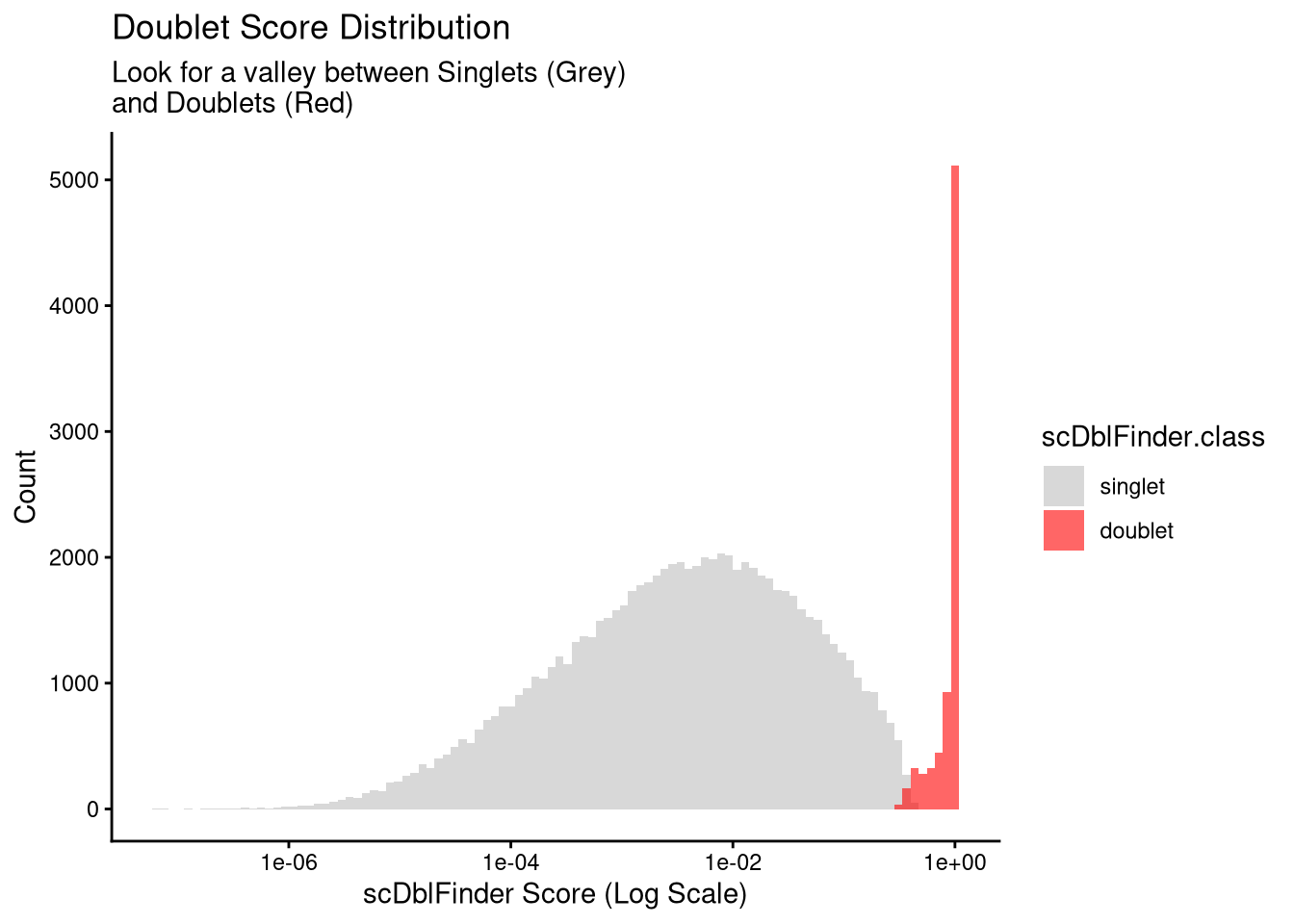
ggsave(file.path(graphs_dir, "QC_scdbl_hist.pdf"), plot = p, width = 12, height = 6, units = "in")Violin plots of UMI counts, feature counts, and mitochondrial percentage split by pool, coloured by scDblFinder classification.
seu_h[["percent.mt"]] <- PercentageFeatureSet(seu_h, pattern = "^MT-")

p <- VlnPlot(
  seu_h,
  features  = c("nCount_RNA", "nFeature_RNA", "percent.mt"),
  group.by  = "pool_id",
  split.by  = "scDblFinder.class",
  pt.size   = 0
) +
  labs(fill = "Cell Class") +
  theme(legend.position = "right")
Warning: Default search for "data" layer in "RNA" assay yielded no results;
utilizing "counts" layer instead.The default behaviour of split.by has changed.
Separate violin plots are now plotted side-by-side.
To restore the old behaviour of a single split violin,
set split.plot = TRUE.
This message will be shown once per session.p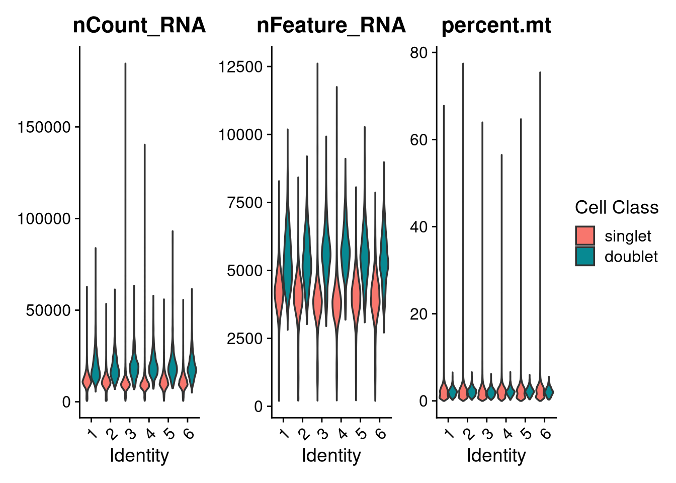
ggsave(file.path(graphs_dir, "QC_scDbl_violin.pdf"), plot = p, width = 12, height = 6, units = "in")plot1 <- FeatureScatter(seu_h, feature1 = "nCount_RNA", feature2 = "percent.mt")
plot2 <- FeatureScatter(seu_h, feature1 = "nCount_RNA", feature2 = "nFeature_RNA")
ggsave(file.path(graphs_dir, "QC_nCount_vs_mt.pdf"), plot = plot1, width = 12, height = 6, units = "in")
ggsave(file.path(graphs_dir, "QC_nCount_vs_feature.pdf"), plot = plot2, width = 12, height = 6, units = "in")
print(plot1)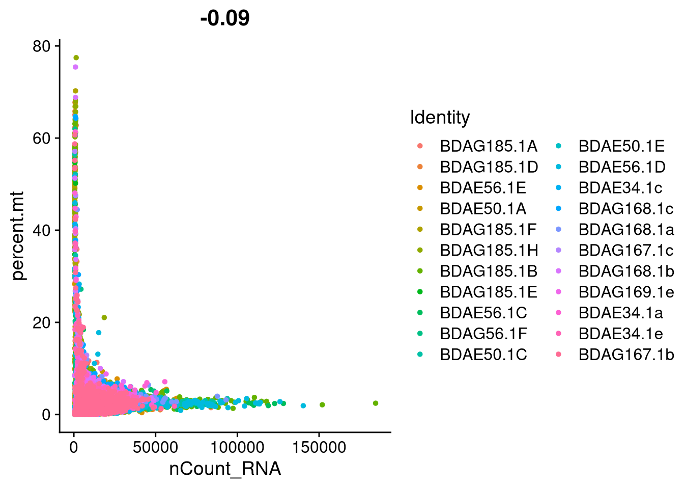
print(plot2)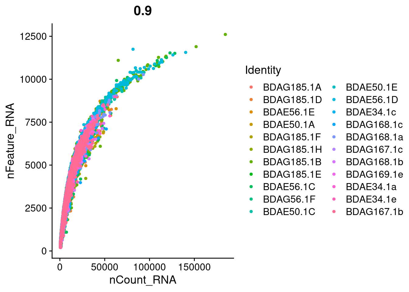
plot <- FeatureScatter(
  seu_h,
  feature1 = "nCount_RNA",
  feature2 = "nFeature_RNA",
  group.by = "scDblFinder.class"
)
ggsave(file.path(graphs_dir, "QC_nCount_vs_feature_doublets.pdf"), plot = plot, width = 12, height = 6, units = "in")
print(plot)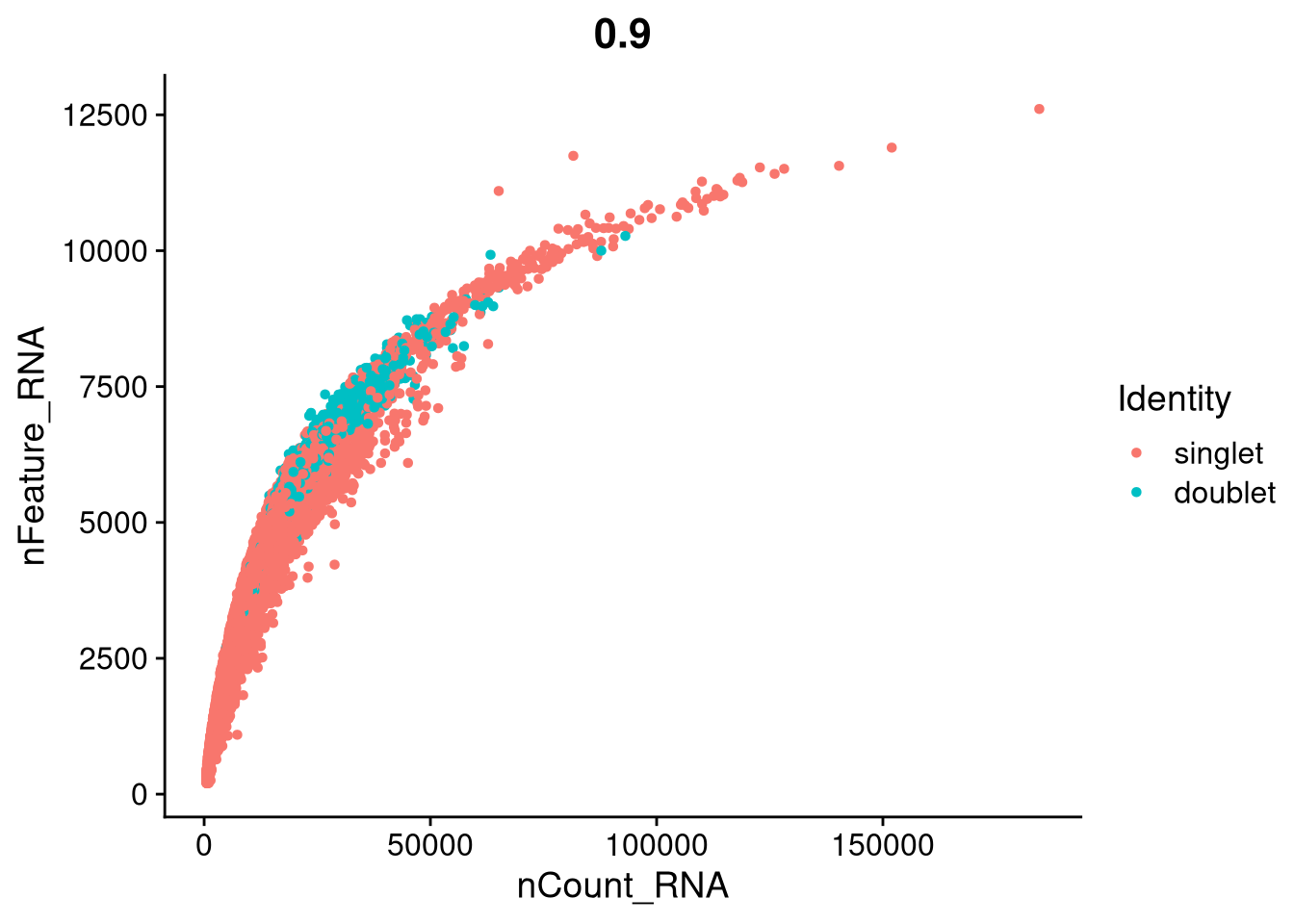
Outliers are flagged using the Median Absolute Deviation (MAD) rather than fixed thresholds, making the cutoff robust to pool-level differences in sequencing depth. Per-pool statistics are calculated and cutoffs at both 3 and 5 MADs above the median are retained for comparison.
seu_h@meta.data <- seu_h@meta.data %>%
  select(-any_of(c("median_count", "mad_count", "upper_limit_5_mad", "upper_limit_3_mad")))

qc_stats <- seu_h@meta.data %>%
  group_by(pool_id) %>%
  summarise(
    median_count = median(nCount_RNA),
    mad_count    = mad(nCount_RNA)
  ) %>%
  mutate(
    upper_limit_5_mad = median_count + (5 * mad_count),
    upper_limit_3_mad = median_count + (3 * mad_count)
  )

meta_updated <- seu_h@meta.data %>%
  rownames_to_column("cell_id") %>%
  left_join(qc_stats, by = "pool_id") %>%
  mutate(
    mad5_outlier = ifelse(nCount_RNA >= upper_limit_5_mad, "Outlier", "Not Outlier"),
    mad3_outlier = ifelse(nCount_RNA >= upper_limit_3_mad, "Outlier", "Not Outlier")
  ) %>%
  column_to_rownames("cell_id")

seu_h@meta.data <- meta_updated

VlnPlot(seu_h, features = "nCount_RNA", group.by = "pool_id", pt.size = 0.1) +
  geom_hline(data = qc_stats, aes(yintercept = upper_limit_5_mad), color = "red", linetype = "dashed")
Warning: Default search for "data" layer in "RNA" assay yielded no results;
utilizing "counts" layer instead.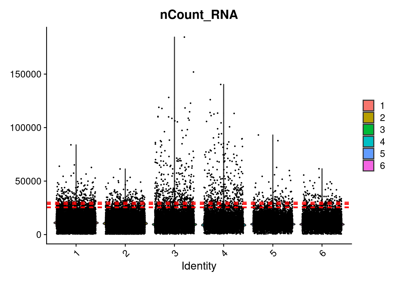
Calculates the number and percentage of cells that would be removed at each MAD threshold, combined with doublet removal.
dbl_col <- "scDblFinder.class"

global_stats <- seu_h@meta.data %>%
  summarise(
    total_cells      = n(),
    n_remove_3       = sum(mad3_outlier == "Outlier" | .data[[dbl_col]] == "doublet"),
    percent_remove_3 = round((n_remove_3 / total_cells) * 100, 2),
    n_remove_5       = sum(mad5_outlier == "Outlier" | .data[[dbl_col]] == "doublet"),
    percent_remove_5 = round((n_remove_5 / total_cells) * 100, 2)
  )

print(global_stats)
total_cells n_remove_3 percent_remove_3 n_remove_5 percent_remove_5
1 88582 9411 10.62 8321 9.39table(Outlier_Status = seu_h$mad3_outlier, Doublet_Status = seu_h$scDblFinder.class) Doublet_Status
Outlier_Status singlet doublet
Not Outlier 79171 4998
Outlier 1791 2622Checks how many cells exceed 6,000 features within each MAD category, as a sanity check against previously used fixed cutoffs.
outlier_summary <- seu_h@meta.data %>%
  group_by(mad3_outlier, mad5_outlier) %>%
  summarise(
    Total_Cells              = n(),
    Cells_Over_6000_Features = sum(nFeature_RNA > 6000),
    Percentage_High_Feature  = round((Cells_Over_6000_Features / Total_Cells) * 100, 2),
    .groups = "drop"
  )

outlier_summaryPrints the number of cells retained or lost at each threshold and overlays both cutoff lines on a violin plot.
counts <- seu_h$nCount_RNA

median_val <- median(counts)
mad_val    <- mad(counts)

cutoff_3mad <- median_val + (3 * mad_val)
cutoff_5mad <- median_val + (5 * mad_val)

cat("Median UMI Count:", median_val, "\n")
Median UMI Count: 10839 cat("MAD:", mad_val, "\n\n")MAD: 3530.071 cat("--- 3 MAD Cutoff ---\n")--- 3 MAD Cutoff ---cat("Threshold:", round(cutoff_3mad, 2), "\n")Threshold: 21429.21 cat("Cells removed:", sum(counts > cutoff_3mad), "\n")Cells removed: 4089 cat("Cells kept:", sum(counts <= cutoff_3mad), "\n\n")Cells kept: 84493 cat("--- 5 MAD Cutoff ---\n")--- 5 MAD Cutoff ---cat("Threshold:", round(cutoff_5mad, 2), "\n")Threshold: 28489.35 cat("Cells removed:", sum(counts > cutoff_5mad), "\n")Cells removed: 1424 cat("Cells kept:", sum(counts <= cutoff_5mad), "\n")Cells kept: 87158 p <- VlnPlot(seu_h, features = "nCount_RNA", pt.size = 0, group.by = "pool_id") +
geom_hline(yintercept = cutoff_3mad, color = "red", linetype = "dashed", size = 1) +
geom_hline(yintercept = cutoff_5mad, color = "blue", linetype = "dashed", size = 1) +
annotate("text", x = 5.1, y = 100000,
label = paste0("3 MAD: ", round(cutoff_3mad)),
vjust = 1.5, hjust = 0, color = "red", fontface = "bold") +
annotate("text", x = 5.1, y = 100000,
label = paste0("5 MAD: ", round(cutoff_5mad)),
vjust = -0.5, hjust = 0, color = "blue", fontface = "bold") +
ggtitle("nCount_RNA Distribution: 3 vs 5 MAD") +
theme(plot.title = element_text(hjust = 0.5)) +
xlab("Pool number") +
ylab("UMI counts")Warning: Default search for "data" layer in "RNA" assay yielded no results;
utilizing "counts" layer instead.Warning: Using `size` aesthetic for lines was deprecated in ggplot2 3.4.0.
ℹ Please use `linewidth` instead.ggsave(
filename = file.path(graphs_dir, glue("count_dist_3_vs_5_mad.pdf")),
plot = p, width = 8, height = 5, dpi = 300, units = "in"
)qc_scatter <- FeatureScatter(seu_h, feature1 = "nCount_RNA", feature2 = "nFeature_RNA",
group.by = "pool_id", shuffle = TRUE) +
geom_vline(xintercept = cutoff_3mad, color = "red", linetype = "dashed", size = 1) +
annotate("text", x = cutoff_3mad, y = max(seu_h$nFeature_RNA), label = "3 MAD",
color = "red", angle = 90, vjust = -0.5, hjust = 1, fontface = "bold") +
geom_vline(xintercept = cutoff_5mad, color = "blue", linetype = "dashed", size = 1) +
annotate("text", x = cutoff_5mad, y = max(seu_h$nFeature_RNA), label = "5 MAD",
color = "blue", angle = 90, vjust = -0.5, hjust = 1, fontface = "bold") +
ggtitle("Count vs Feature (with MAD Cutoffs)") +
xlab("Number of counts") +
ylab("Number of genes")
ggsave(
filename = file.path(graphs_dir, "QC_count_vs_feat_lines.pdf"),
plot = qc_scatter, width = 7, height = 5, dpi = 300, units = "in"
)
print(qc_scatter)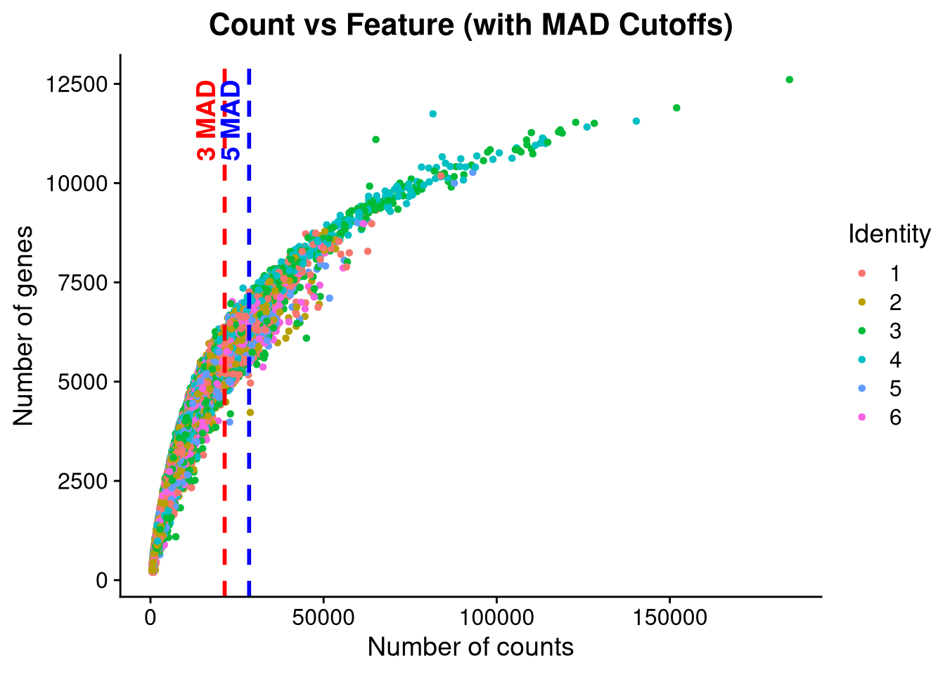
Cells are filtered on three criteria: fewer than 500 detected genes, mitochondrial content above 15%, or flagged as a MAD5 outlier. Doublets are retained here and removed in Part 2 once cluster identity has been confirmed.
ncol(seu_h)[1] 88582seu_h_f <- subset(seu_h, subset = nFeature_RNA > 500 & percent.mt < 15 & mad5_outlier != "Outlier")
ncol(seu_h_f)[1] 86504qs_save(seu_h_f, file.path(objects_dir, "seu_h_initial_subset.qs2"))A quick unintegrated UMAP gives an initial view of structure and reveals whether pool-level batch effects require correction.
options(future.globals.maxSize = 65 * 1024^3)
seu_h_f <- SCTransform(seu_h_f, vst.flavor = "v2", verbose = FALSE)
seu_h_f <- RunPCA(seu_h_f)
PC_ 1
Positive: P2RY12, XACT, PLXDC2, OLR1, SPP1, IFNGR1, CX3CR1, FRMD4A, DOCK4, APBB1IP
CD69, HTRA1, IPCEF1, C3, APOC2, FCGR3A, LINC02712, ENSG00000249738, P2RY13, RGS1
SAMSN1, ADAM28, CCDC200, OLFML3, SRGN, SORL1, DLEU1, FYB1, SIPA1L2, ST6GAL1
Negative: RNASE1, SELENOP, CD36, LYVE1, F13A1, DAB2, COLEC12, CD163, SCN9A, PID1
MRC1, CD163L1, IGFBP4, TGFBI, LILRB5, IQGAP2, ITSN1, CCL8, VAV3, CD200R1
CD28, FGF13, WWP1, RND3, ANTXR2, NRP1, MS4A4A, CCDC170, CCL2, RBPJ
PC_ 2
Positive: SPP1, HLA-DRA, CD9, APOC1, FTL, FTH1, EEF1A1, CD74, TPT1, HLA-DPA1
HLA-DRB1, RPL34, HLA-DPB1, NAP1L1, TMSB4X, RPS8, LGALS3, RPL13, RPL10, APOE
CCL4L2, PLA2G7, RPS24, RPS14, RPL5, RPL41, RPL13A, CCL3, CCL4, GPNMB
Negative: MKI67, TOP2A, CENPF, ASPM, TPX2, HMMR, KNL1, NUSAP1, ANLN, CDK1
PRC1, UBE2C, H1-5, DLGAP5, NDC80, DIAPH3, GTSE1, NCAPG, KIF14, CENPE
RRM2, CKAP2L, HMGB2, CCNA2, CDCA2, H2AC14, CEP55, SYNE2, KIF23, TYMS
PC_ 3
Positive: FRMD4A, SFMBT2, DOCK4, ITPR2, AFF3, SLC9A9, ENSG00000249738, MEF2A, P2RY12, AOAH
SMYD3, LRMDA, KCNQ3, FCHSD2, PLXDC2, LINC02712, FOXN3, QKI, DIAPH2, SSBP2
LYVE1, ELMO1, SLC8A1, PRKCA, MAML2, ST6GAL1, SRGAP2, ZSWIM6, ENSG00000231918, MERTK
Negative: SPP1, HLA-DRA, CD9, APOC1, HLA-DPA1, FTL, HLA-DRB1, FTH1, TMSB4X, CD74
NAP1L1, HLA-DPB1, LGALS1, EEF1A1, TPT1, RPS8, LGALS3, DBI, CCL4, RPLP1
RPL13, RPS2, APOE, CCL3, PLA2G7, RPL41, RPL10, RPS6, GPNMB, RPS24
PC_ 4
Positive: MT-CO1, MT-CO3, MT-ND4, MT-CO2, TMSB4X, MT-CYB, MT-ATP6, TPT1, MT-ND3, RPLP1
RPS8, RPL13, MT-ND5, RPS24, EEF1A1, MT-ND4L, RPL13A, MT-ND2, FTL, ENSG00000289901
RPS2, RPS4X, RPS23, RPL34, RPS14, AIF1, MT-ND1, RPL21, P2RY12, RPS6
Negative: CCL4, CCL4L2, CCL3, CCL3L3, FOS, IL1B, DUSP1, GADD45B, CCDC200, SPP1
CCL2, TEX14, IER2, NR4A2, CD83, KLF2, CD69, BTG2, SRGN, JUNB
JUN, CXCL8, IER3, ENSG00000262202, CD36, NR4A1, OLR1, ZFP36, EGR1, ATF3
PC_ 5
Positive: CCDC200, CCL4L2, TEX14, ENSG00000262202, TPT1, AGR2, ENSG00000285646, NR4A1, PTH2R, LYVE1
CCL3L3, CST3, EEF1A1, PNRC1, RPL13, ENSG00000287979, IER3, FOSB, NR4A2, RPL13A
LINC00910, RPS8, RPS24, IER2, AIF1, IL1B, BTG2, RPLP1, H3-3B, RPL41
Negative: SPP1, CD9, IFIT3, APOC1, MX1, IFIT1, IFI44L, IFI6, IFIT2, GPNMB
LGALS3, LGALS1, IFI27, XACT, APOE, IFITM1, MX2, RTTN, GLDN, RSAD2
SCIN, MYO1E, PLA2G7, RGCC, ISG15, LINC01235, MSR1, LIPA, PLXDC2, IFITM3 seu_h_f <- RunUMAP(seu_h_f, dims = 1:30)Warning: The default method for RunUMAP has changed from calling Python UMAP via reticulate to the R-native UWOT using the cosine metric
To use Python UMAP via reticulate, set umap.method to 'umap-learn' and metric to 'correlation'
This message will be shown once per session17:42:47 UMAP embedding parameters a = 0.9922 b = 1.11217:42:47 Read 86504 rows and found 30 numeric columns17:42:47 Using Annoy for neighbor search, n_neighbors = 3017:42:47 Building Annoy index with metric = cosine, n_trees = 500% 10 20 30 40 50 60 70 80 90 100%[----|----|----|----|----|----|----|----|----|----|**************************************************|
17:42:53 Writing NN index file to temp file /tmp/slurm_45934587/RtmpfBZYPK/filedc5153069a22
17:42:53 Searching Annoy index using 1 thread, search_k = 3000
17:43:22 Annoy recall = 100%
17:43:24 Commencing smooth kNN distance calibration using 1 thread with target n_neighbors = 30
17:43:29 Initializing from normalized Laplacian + noise (using RSpectra)
17:43:34 Commencing optimization for 200 epochs, with 3929318 positive edges
17:43:34 Using rng type: pcg
17:44:14 Optimization finishedp <- DimPlot(seu_h_f,
reduction = "umap",
split.by = "pool_id",
group.by = "pool_id") +
ggtitle("Unintegrated Data: Split by Pool")
p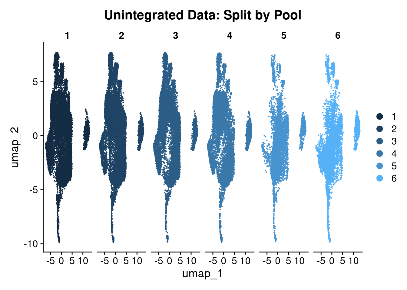
ggsave(file.path(graphs_dir, "QC_umaps_pools_split.pdf"), plot = p, width = 18, height = 6, units = "in")Each pool is processed independently to assess quality and score cell type identity before integration. This allows per-pool QC inspection and ensures Mancuso signatures are applied at the batch level.
Gene sets for non-microglial cell types (provided by Emma) and Mancuso 2024 microglial states are loaded here for use in both batch-level and integrated scoring.
sig_dir <- file.path(base_dir, "signatures")

gs_myeloid       <- readLines(file.path(sig_dir, "myeloid.txt"))
gs_proliferating <- readLines(file.path(sig_dir, "proliferating.txt"))
gs_macrophage    <- readLines(file.path(sig_dir, "macrophage.txt"))
gs_dendritic     <- readLines(file.path(sig_dir, "dendritic.txt"))

mancuso_dir <- "/nemo/lab/destrooperb/home/shared/zanettc/Mancuso2024_genesets"

gs_crm  <- readLines(file.path(mancuso_dir, "CRM_geneset.txt"))
gs_dam  <- readLines(file.path(mancuso_dir, "DAM_geneset.txt"))
gs_hla  <- readLines(file.path(mancuso_dir, "HLA_geneset.txt"))
gs_hm   <- readLines(file.path(mancuso_dir, "HM_geneset.txt"))
gs_irm  <- readLines(file.path(mancuso_dir, "IRM_geneset.txt"))
gs_rm   <- readLines(file.path(mancuso_dir, "RM_geneset.txt"))
Warning in readLines(file.path(mancuso_dir, "RM_geneset.txt")): incomplete
final line found on
'/nemo/lab/destrooperb/home/shared/zanettc/Mancuso2024_genesets/RM_geneset.txt'gs_tcrm <- readLines(file.path(mancuso_dir, "transCRM_geneset.txt"))Each batch is normalised with SCTransform, reduced with PCA, and embedded with UMAP. Clustering at resolution 0.2 generates initial cluster assignments for module scoring.
batches <- SplitObject(seu_h_f, split.by = "pool_id")

options(future.globals.maxSize = 8912896000000)
batches <- lapply(batches, SCTransform)
Running SCTransform on assay: RNAvst.flavor='v2' set. Using model with fixed slope and excluding poisson genes.Calculating cell attributes from input UMI matrix: log_umiVariance stabilizing transformation of count matrix of size 24322 by 18350Model formula is y ~ log_umiGet Negative Binomial regression parameters per geneUsing 2000 genes, 5000 cellsFound 196 outliers - those will be ignored in fitting/regularization stepSecond step: Get residuals using fitted parameters for 24322 genesComputing corrected count matrix for 24322 genesCalculating gene attributesWall clock passed: Time difference of 1.362898 minsDetermine variable featuresCentering data matrixPlace corrected count matrix in counts slotWarning: Different cells and/or features from existing assay SCTSet default assay to SCTRunning SCTransform on assay: RNAvst.flavor='v2' set. Using model with fixed slope and excluding poisson genes.Calculating cell attributes from input UMI matrix: log_umiVariance stabilizing transformation of count matrix of size 24054 by 18346Model formula is y ~ log_umiGet Negative Binomial regression parameters per geneUsing 2000 genes, 5000 cellsFound 225 outliers - those will be ignored in fitting/regularization stepSecond step: Get residuals using fitted parameters for 24054 genesComputing corrected count matrix for 24054 genesCalculating gene attributesWall clock passed: Time difference of 1.339851 minsDetermine variable featuresCentering data matrixPlace corrected count matrix in counts slotWarning: Different cells and/or features from existing assay SCTSet default assay to SCTRunning SCTransform on assay: RNAvst.flavor='v2' set. Using model with fixed slope and excluding poisson genes.Calculating cell attributes from input UMI matrix: log_umiVariance stabilizing transformation of count matrix of size 23159 by 16345Model formula is y ~ log_umiGet Negative Binomial regression parameters per geneUsing 2000 genes, 5000 cellsFound 199 outliers - those will be ignored in fitting/regularization stepSecond step: Get residuals using fitted parameters for 23159 genesComputing corrected count matrix for 23159 genesCalculating gene attributesWall clock passed: Time difference of 1.183697 minsDetermine variable featuresCentering data matrixPlace corrected count matrix in counts slotWarning: Different cells and/or features from existing assay SCTSet default assay to SCTRunning SCTransform on assay: RNAvst.flavor='v2' set. Using model with fixed slope and excluding poisson genes.Calculating cell attributes from input UMI matrix: log_umiVariance stabilizing transformation of count matrix of size 22383 by 10620Model formula is y ~ log_umiGet Negative Binomial regression parameters per geneUsing 2000 genes, 5000 cellsFound 158 outliers - those will be ignored in fitting/regularization stepSecond step: Get residuals using fitted parameters for 22383 genesComputing corrected count matrix for 22383 genesCalculating gene attributesWall clock passed: Time difference of 49.21991 secsDetermine variable featuresCentering data matrixPlace corrected count matrix in counts slotWarning: Different cells and/or features from existing assay SCTSet default assay to SCTRunning SCTransform on assay: RNAvst.flavor='v2' set. Using model with fixed slope and excluding poisson genes.Calculating cell attributes from input UMI matrix: log_umiVariance stabilizing transformation of count matrix of size 22633 by 10588Model formula is y ~ log_umiGet Negative Binomial regression parameters per geneUsing 2000 genes, 5000 cellsFound 154 outliers - those will be ignored in fitting/regularization stepSecond step: Get residuals using fitted parameters for 22633 genesComputing corrected count matrix for 22633 genesCalculating gene attributesWall clock passed: Time difference of 51.41714 secsDetermine variable featuresCentering data matrixPlace corrected count matrix in counts slotWarning: Different cells and/or features from existing assay SCTSet default assay to SCTRunning SCTransform on assay: RNAvst.flavor='v2' set. Using model with fixed slope and excluding poisson genes.Calculating cell attributes from input UMI matrix: log_umiVariance stabilizing transformation of count matrix of size 23243 by 12255Model formula is y ~ log_umiGet Negative Binomial regression parameters per geneUsing 2000 genes, 5000 cellsFound 175 outliers - those will be ignored in fitting/regularization stepSecond step: Get residuals using fitted parameters for 23243 genesComputing corrected count matrix for 23243 genesCalculating gene attributesWall clock passed: Time difference of 56.26383 secsDetermine variable featuresCentering data matrixPlace corrected count matrix in counts slotWarning: Different cells and/or features from existing assay SCTSet default assay to SCTbatches <- lapply(batches, \(o) {
set.seed(42)
o <- RunPCA(o, npcs = 30, assay = "SCT", verbose = FALSE)
set.seed(42)
o <- RunUMAP(o, dims = 1:25, n.neighbors = 30L, n.epochs = 500, min.dist = 0.05)
o
})Warning: Number of dimensions changing from 50 to 3017:51:55 UMAP embedding parameters a = 1.75 b = 0.842117:51:55 Read 18350 rows and found 25 numeric columns17:51:55 Using Annoy for neighbor search, n_neighbors = 3017:51:55 Building Annoy index with metric = cosine, n_trees = 500% 10 20 30 40 50 60 70 80 90 100%[----|----|----|----|----|----|----|----|----|----|**************************************************|
17:51:56 Writing NN index file to temp file /tmp/slurm_45934587/RtmpfBZYPK/filedc51518aba28f
17:51:56 Searching Annoy index using 1 thread, search_k = 3000
17:52:01 Annoy recall = 100%
17:52:03 Commencing smooth kNN distance calibration using 1 thread with target n_neighbors = 30
17:52:06 Initializing from normalized Laplacian + noise (using RSpectra)
17:52:07 Commencing optimization for 500 epochs, with 798570 positive edges
17:52:07 Using rng type: pcg
17:52:28 Optimization finishedWarning: Number of dimensions changing from 50 to 3017:52:33 UMAP embedding parameters a = 1.75 b = 0.8421
17:52:33 Read 18346 rows and found 25 numeric columns
17:52:33 Using Annoy for neighbor search, n_neighbors = 30
17:52:33 Building Annoy index with metric = cosine, n_trees = 50
0% 10 20 30 40 50 60 70 80 90 100%
[----|----|----|----|----|----|----|----|----|----|
**************************************************|
17:52:35 Writing NN index file to temp file /tmp/slurm_45934587/RtmpfBZYPK/filedc515249d6a3f
17:52:35 Searching Annoy index using 1 thread, search_k = 3000
17:52:39 Annoy recall = 100%
17:52:41 Commencing smooth kNN distance calibration using 1 thread with target n_neighbors = 30
17:52:45 Initializing from normalized Laplacian + noise (using RSpectra)
17:52:45 Commencing optimization for 500 epochs, with 815792 positive edges
17:52:45 Using rng type: pcg
17:53:06 Optimization finishedWarning: Number of dimensions changing from 50 to 3017:53:11 UMAP embedding parameters a = 1.75 b = 0.8421
17:53:11 Read 16345 rows and found 25 numeric columns
17:53:11 Using Annoy for neighbor search, n_neighbors = 30
17:53:11 Building Annoy index with metric = cosine, n_trees = 50
0% 10 20 30 40 50 60 70 80 90 100%
[----|----|----|----|----|----|----|----|----|----|
**************************************************|
17:53:12 Writing NN index file to temp file /tmp/slurm_45934587/RtmpfBZYPK/filedc51573057ced
17:53:12 Searching Annoy index using 1 thread, search_k = 3000
17:53:16 Annoy recall = 100%
17:53:18 Commencing smooth kNN distance calibration using 1 thread with target n_neighbors = 30
17:53:22 Initializing from normalized Laplacian + noise (using RSpectra)
17:53:22 Commencing optimization for 500 epochs, with 718316 positive edges
17:53:22 Using rng type: pcg
17:53:41 Optimization finishedWarning: Number of dimensions changing from 50 to 3017:53:45 UMAP embedding parameters a = 1.75 b = 0.8421
17:53:45 Read 10620 rows and found 25 numeric columns
17:53:45 Using Annoy for neighbor search, n_neighbors = 30
17:53:45 Building Annoy index with metric = cosine, n_trees = 50
0% 10 20 30 40 50 60 70 80 90 100%
[----|----|----|----|----|----|----|----|----|----|
**************************************************|
17:53:45 Writing NN index file to temp file /tmp/slurm_45934587/RtmpfBZYPK/filedc51584005a9
17:53:45 Searching Annoy index using 1 thread, search_k = 3000
17:53:48 Annoy recall = 100%
17:53:49 Commencing smooth kNN distance calibration using 1 thread with target n_neighbors = 30
17:53:53 Initializing from normalized Laplacian + noise (using RSpectra)
17:53:53 Commencing optimization for 500 epochs, with 460334 positive edges
17:53:53 Using rng type: pcg
17:54:06 Optimization finishedWarning: Number of dimensions changing from 50 to 3017:54:09 UMAP embedding parameters a = 1.75 b = 0.8421
17:54:09 Read 10588 rows and found 25 numeric columns
17:54:09 Using Annoy for neighbor search, n_neighbors = 30
17:54:09 Building Annoy index with metric = cosine, n_trees = 50
0% 10 20 30 40 50 60 70 80 90 100%
[----|----|----|----|----|----|----|----|----|----|
**************************************************|
17:54:10 Writing NN index file to temp file /tmp/slurm_45934587/RtmpfBZYPK/filedc51573561cc9
17:54:10 Searching Annoy index using 1 thread, search_k = 3000
17:54:13 Annoy recall = 100%
17:54:14 Commencing smooth kNN distance calibration using 1 thread with target n_neighbors = 30
17:54:18 Initializing from normalized Laplacian + noise (using RSpectra)
17:54:18 Commencing optimization for 500 epochs, with 460154 positive edges
17:54:18 Using rng type: pcg
17:54:31 Optimization finishedWarning: Number of dimensions changing from 50 to 3017:54:35 UMAP embedding parameters a = 1.75 b = 0.8421
17:54:35 Read 12255 rows and found 25 numeric columns
17:54:35 Using Annoy for neighbor search, n_neighbors = 30
17:54:35 Building Annoy index with metric = cosine, n_trees = 50
0% 10 20 30 40 50 60 70 80 90 100%
[----|----|----|----|----|----|----|----|----|----|
**************************************************|
17:54:36 Writing NN index file to temp file /tmp/slurm_45934587/RtmpfBZYPK/filedc5156a84bc96
17:54:36 Searching Annoy index using 1 thread, search_k = 3000
17:54:39 Annoy recall = 100%
17:54:40 Commencing smooth kNN distance calibration using 1 thread with target n_neighbors = 30
17:54:44 Initializing from normalized Laplacian + noise (using RSpectra)
17:54:44 Commencing optimization for 500 epochs, with 529934 positive edges
17:54:44 Using rng type: pcg
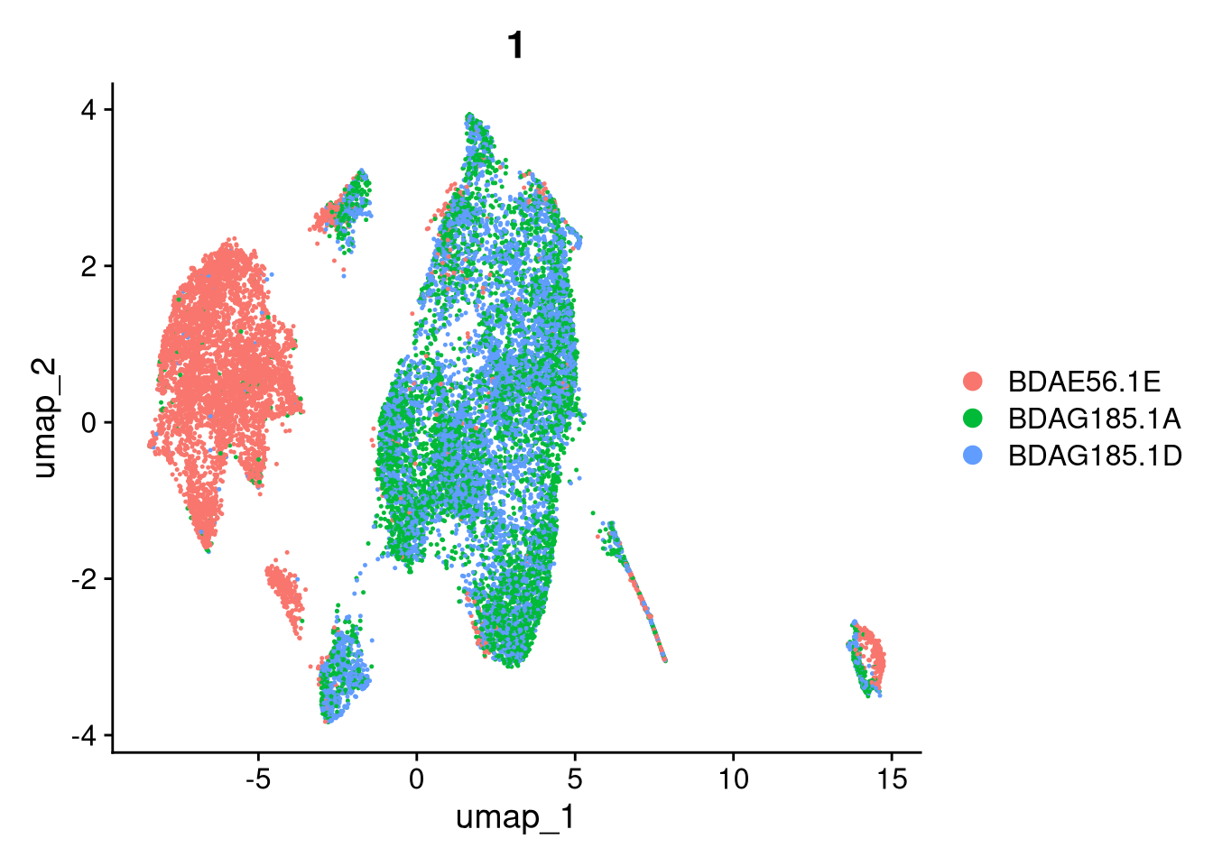
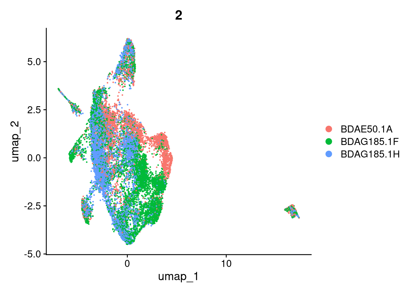
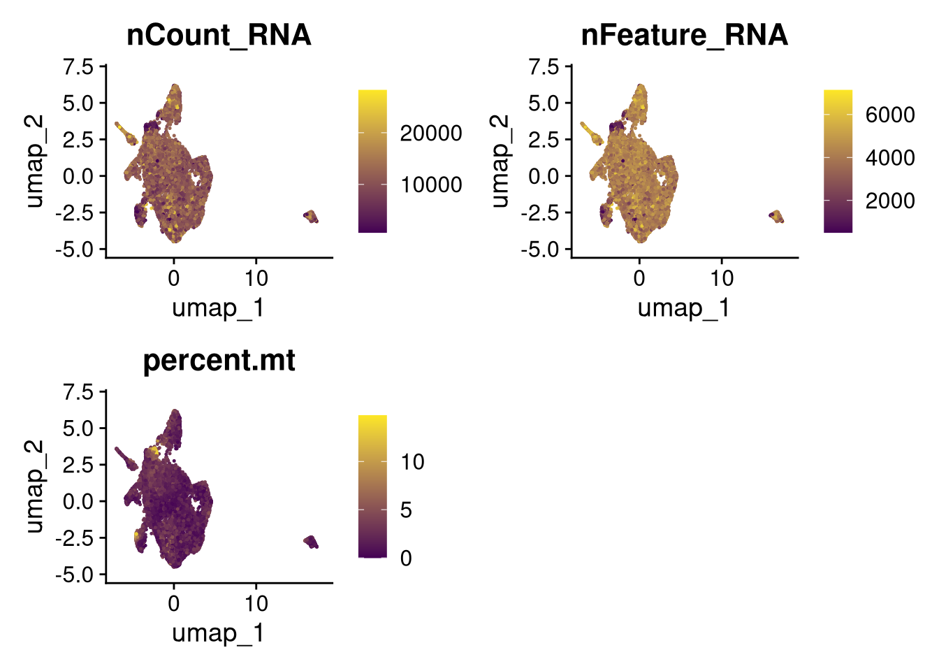
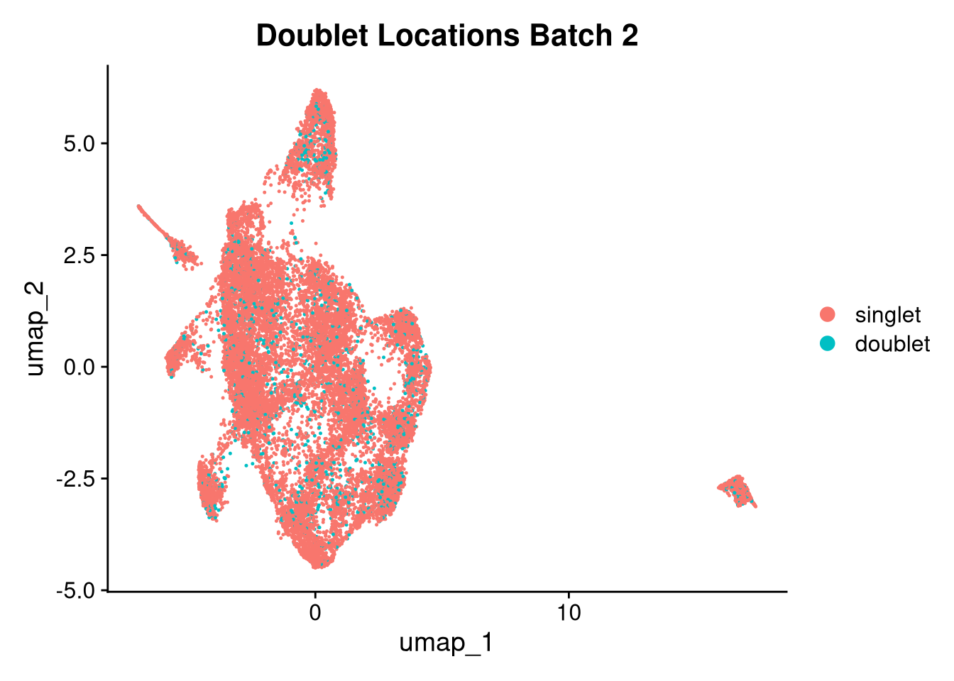
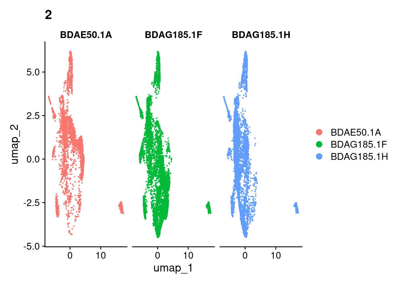
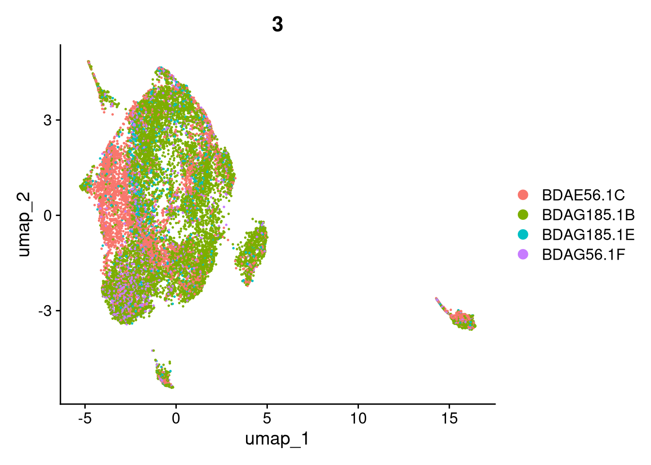
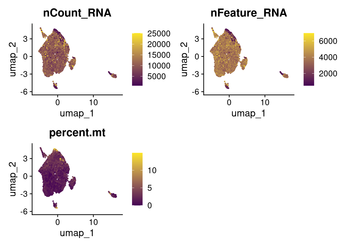
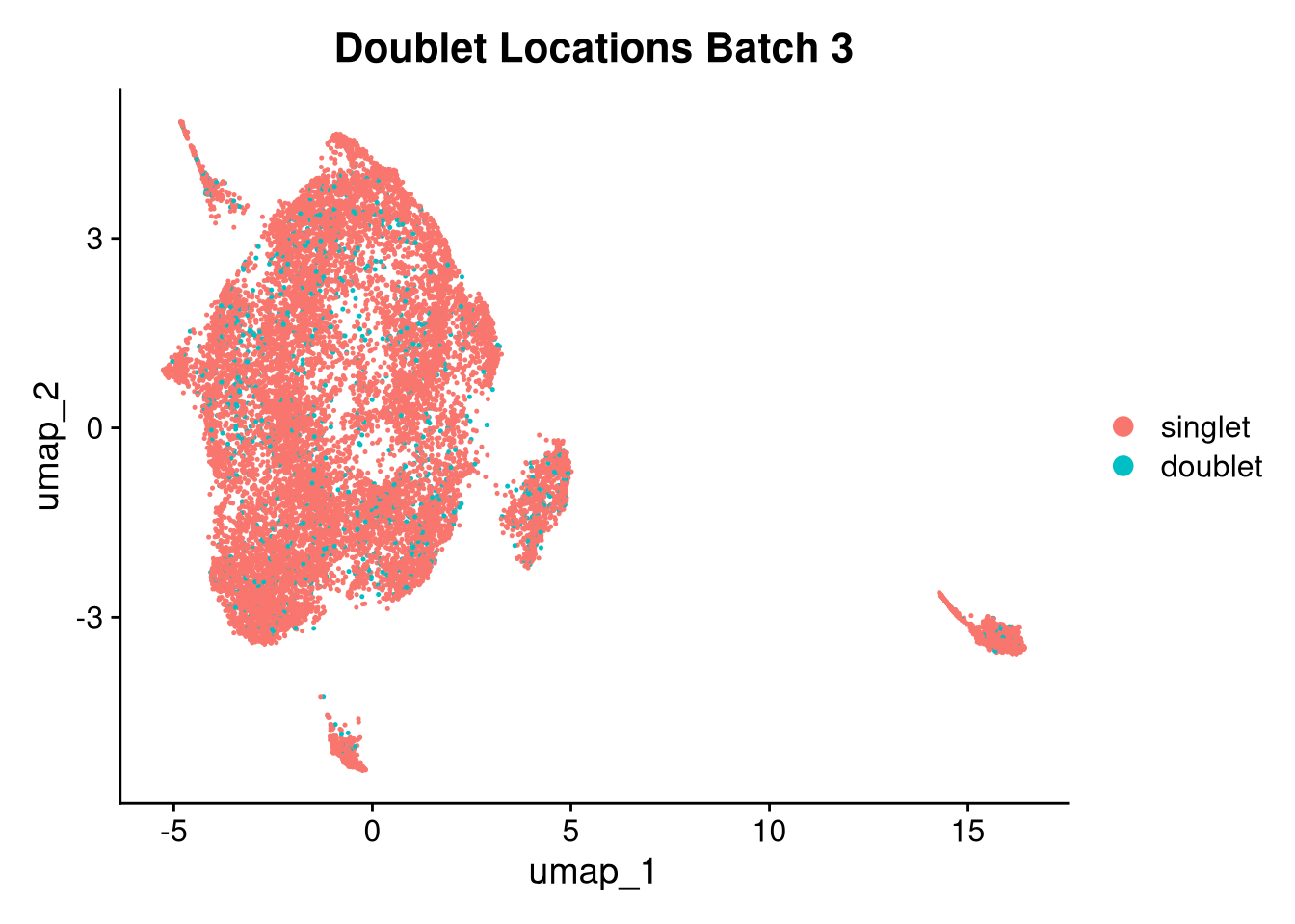
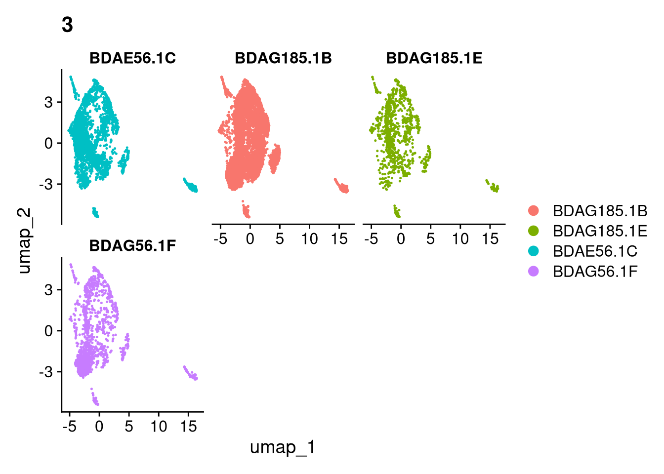
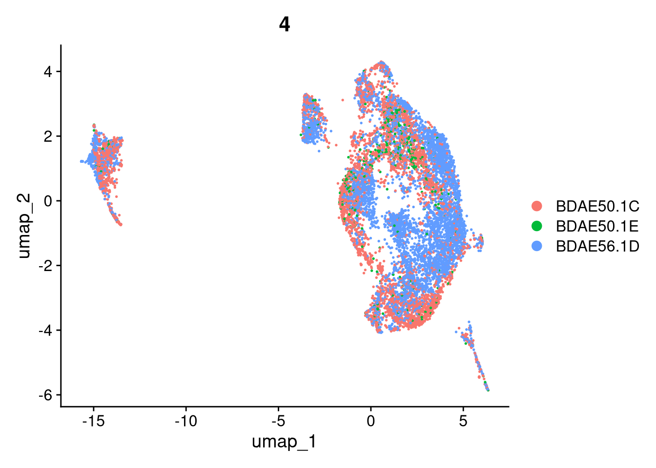
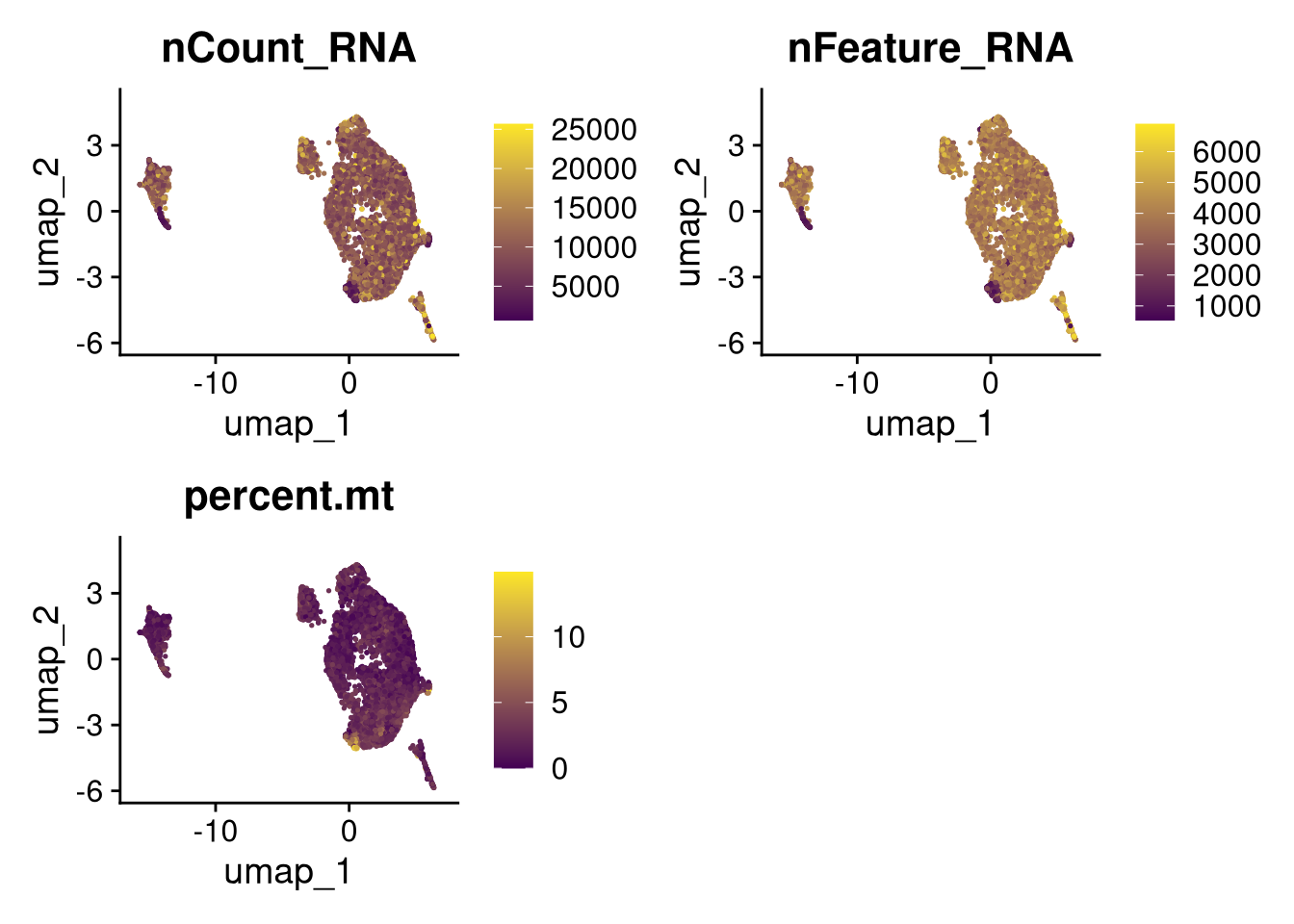
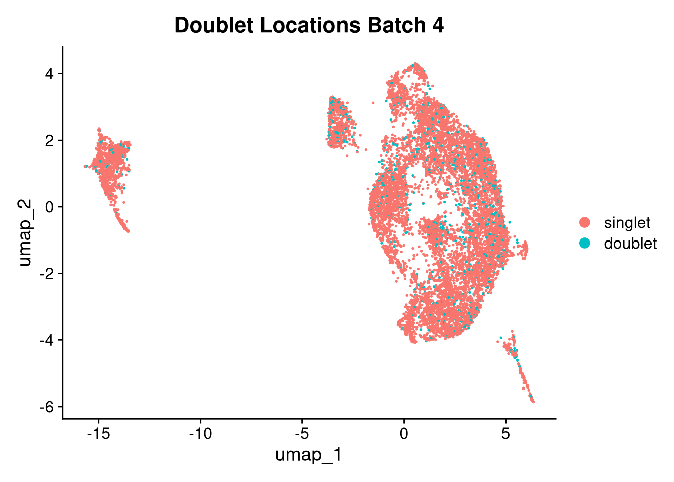
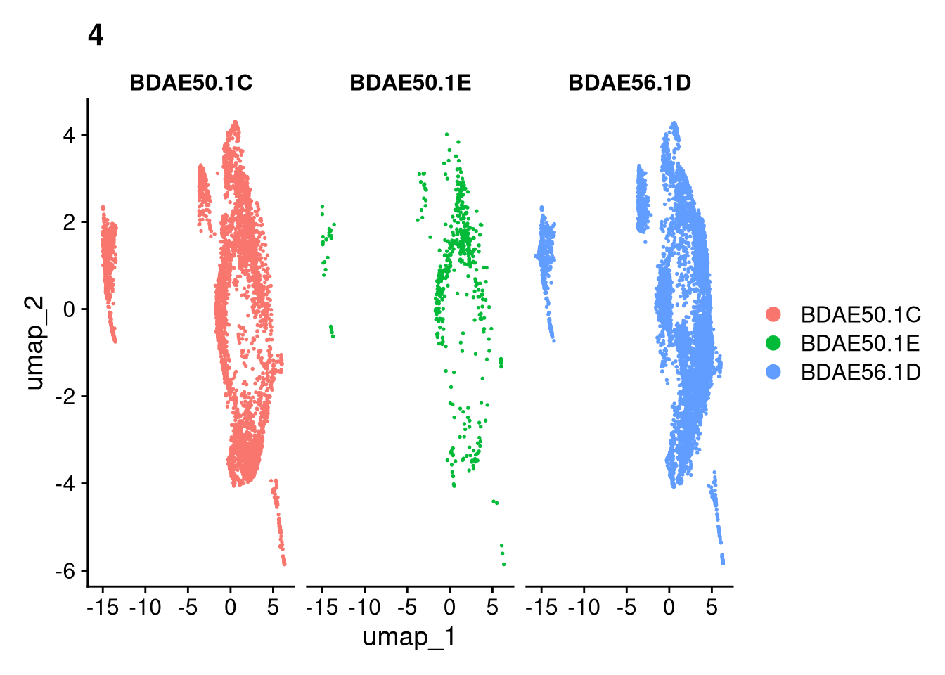
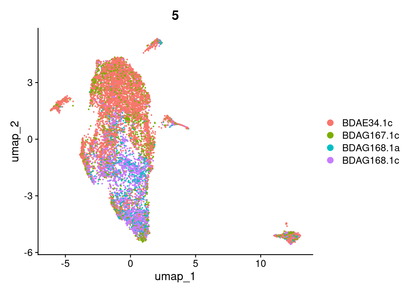
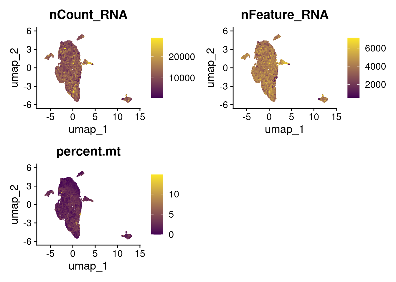
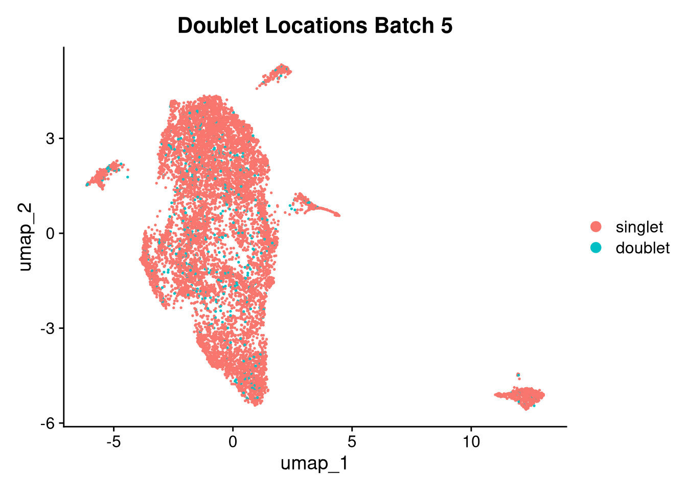
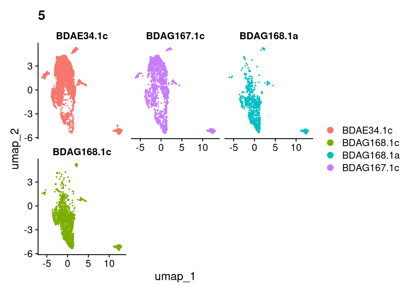
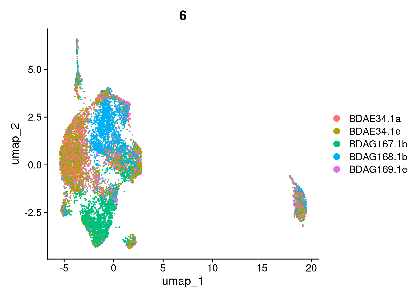
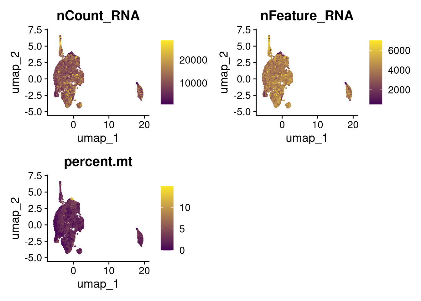
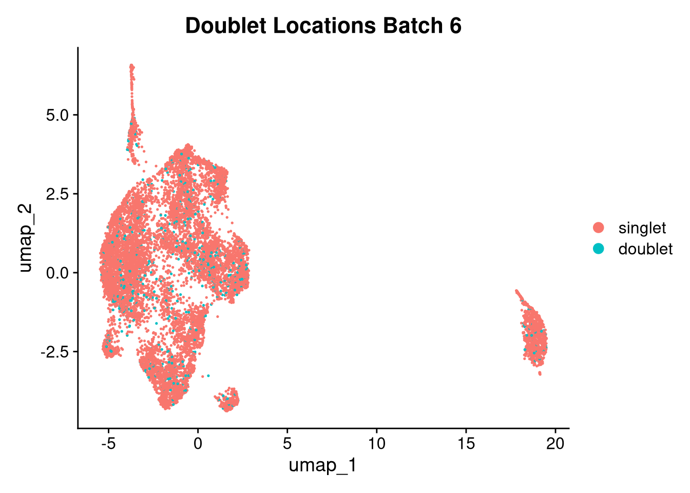
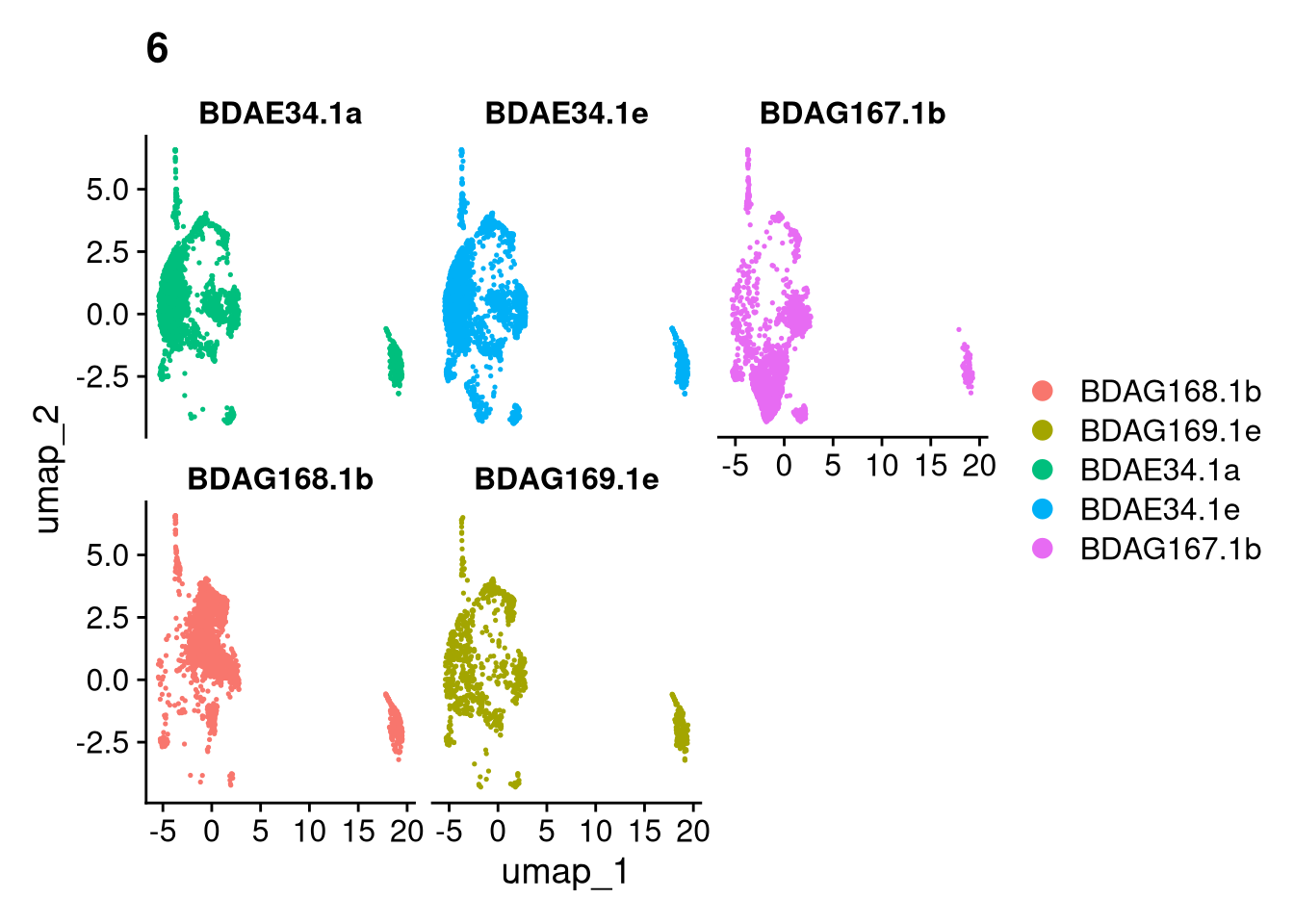
17:54:59 Optimization finishedinvisible(lapply(names(batches), function(nm) {
p <- DimPlot(batches[[nm]], reduction = "umap", group.by = "orig.ident", shuffle = TRUE) + ggtitle(nm)
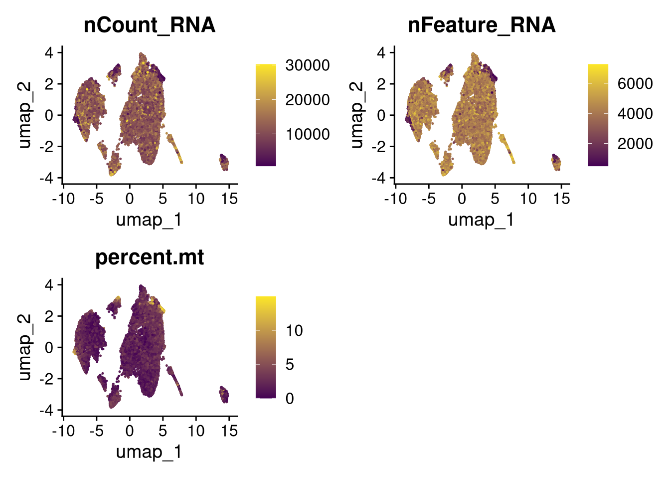
p2 <- FeaturePlot(batches[[nm]], features = c("nCount_RNA", "nFeature_RNA", "percent.mt"), cols = c("#440154", "#FDE725"))
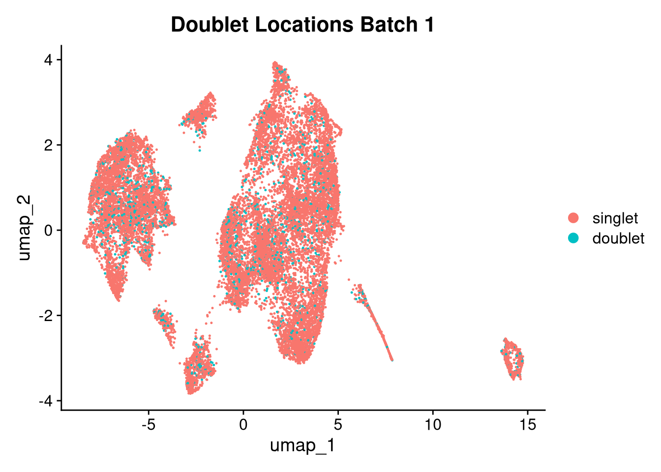
p3 <- DimPlot(batches[[nm]], group.by = "scDblFinder.class") + ggtitle(glue("Doublet Locations Batch {nm}"))
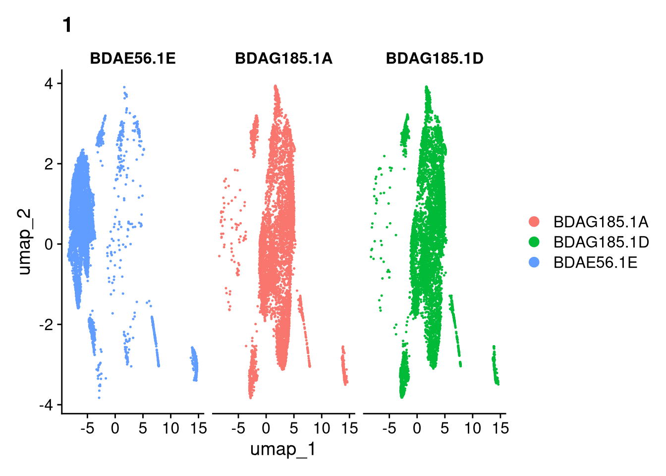
p4 <- DimPlot(batches[[nm]], reduction = "umap", split.by = "orig.ident", shuffle = TRUE, ncol = 3) + ggtitle(nm)
print(p); print(p2); print(p3); print(p4)
batch_graphs_dir <- file.path(graphs_dir, glue("batch_{nm}"))
dir.create(batch_graphs_dir, recursive = TRUE, showWarnings = FALSE)
ggsave(filename = file.path(batch_graphs_dir, glue("QC_batch{nm}_umap_samples_overlayed.pdf")), plot = p, width = 7, height = 5, dpi = 300, units = "in")
ggsave(filename = file.path(batch_graphs_dir, glue("QC_batch{nm}_umap_qc_x3.pdf")), plot = p2, width = 7, height = 5, dpi = 300, units = "in")
ggsave(filename = file.path(batch_graphs_dir, glue("QC_batch{nm}_doublets_umap.pdf")), plot = p3, width = 7, height = 5, dpi = 300, units = "in")
ggsave(filename = file.path(batch_graphs_dir, glue("QC_batch{nm}_umap_samples_split.pdf")), plot = p4, width = 7, height = 5, dpi = 300, units = "in")
}))
qs_save(batches, file = file.path(objects_dir, "umap_batches.qs2"))batches <- qs_read(file.path(objects_dir, "umap_batches.qs2"))res <- 0.2
batches <- lapply(batches, \(o) {
set.seed(42)
o <- FindNeighbors(o, reduction = "pca", dims = 1:30)
set.seed(42)
o <- FindClusters(o, resolution = res)
})Computing nearest neighbor graphComputing SNNModularity Optimizer version 1.3.0 by Ludo Waltman and Nees Jan van Eck
Number of nodes: 18350
Number of edges: 608878
Running Louvain algorithm...
Maximum modularity in 10 random starts: 0.9067
Number of communities: 8
Elapsed time: 3 secondsComputing nearest neighbor graph
Computing SNNModularity Optimizer version 1.3.0 by Ludo Waltman and Nees Jan van Eck
Number of nodes: 18346
Number of edges: 614514
Running Louvain algorithm...
Maximum modularity in 10 random starts: 0.8986
Number of communities: 9
Elapsed time: 2 secondsComputing nearest neighbor graph
Computing SNNModularity Optimizer version 1.3.0 by Ludo Waltman and Nees Jan van Eck
Number of nodes: 16345
Number of edges: 521575
Running Louvain algorithm...
Maximum modularity in 10 random starts: 0.8821
Number of communities: 8
Elapsed time: 2 secondsComputing nearest neighbor graph
Computing SNNModularity Optimizer version 1.3.0 by Ludo Waltman and Nees Jan van Eck
Number of nodes: 10620
Number of edges: 360281
Running Louvain algorithm...
Maximum modularity in 10 random starts: 0.8946
Number of communities: 8
Elapsed time: 1 secondsComputing nearest neighbor graph
Computing SNNModularity Optimizer version 1.3.0 by Ludo Waltman and Nees Jan van Eck
Number of nodes: 10588
Number of edges: 344063
Running Louvain algorithm...
Maximum modularity in 10 random starts: 0.8836
Number of communities: 7
Elapsed time: 1 secondsComputing nearest neighbor graph
Computing SNNModularity Optimizer version 1.3.0 by Ludo Waltman and Nees Jan van Eck
Number of nodes: 12255
Number of edges: 406332
Running Louvain algorithm...
Maximum modularity in 10 random starts: 0.8973
Number of communities: 8
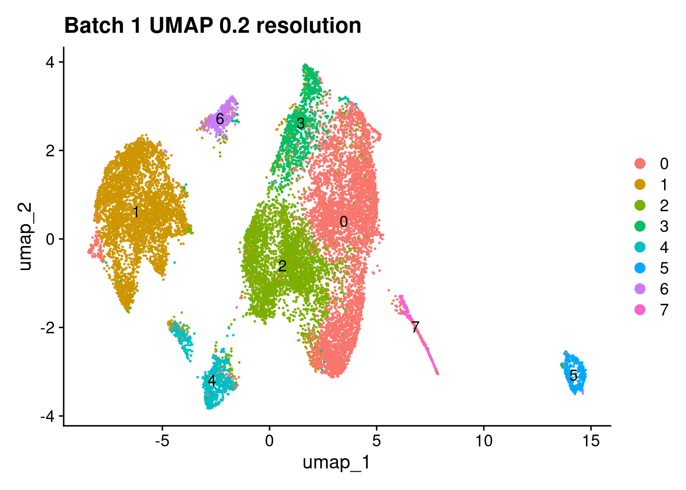
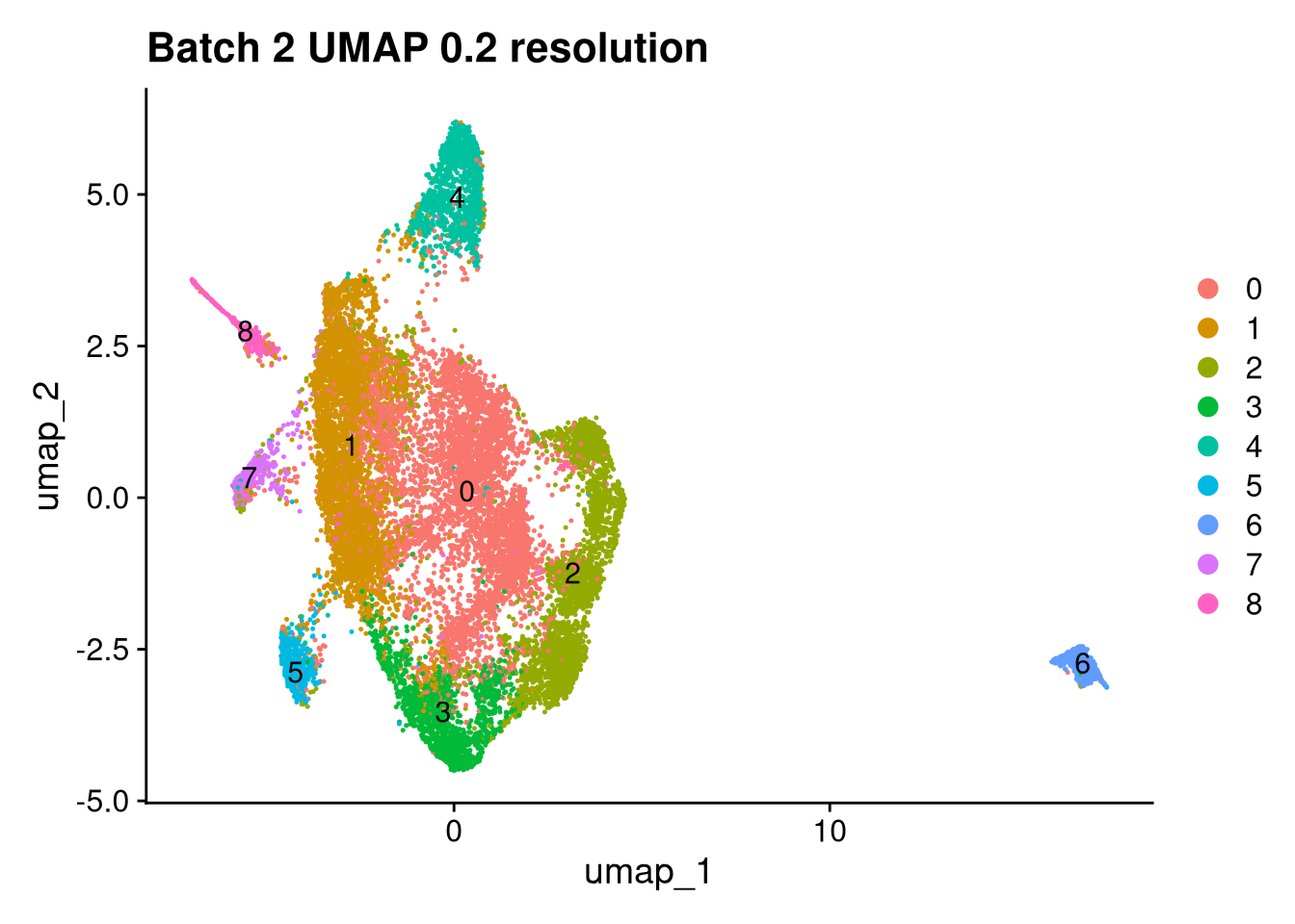
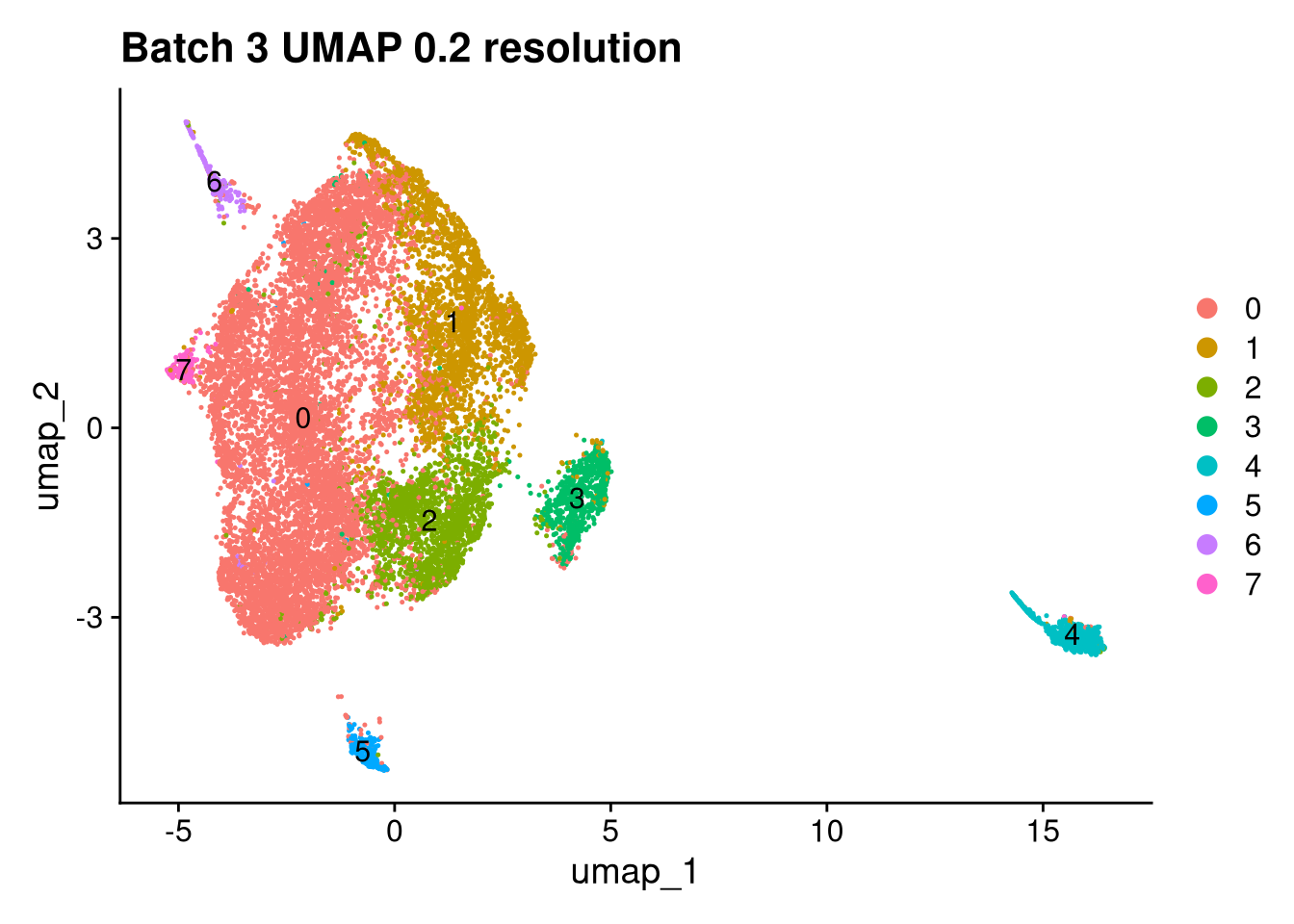
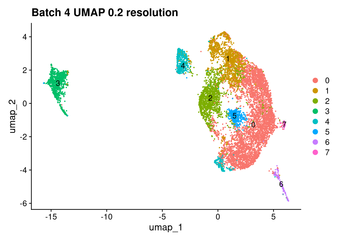
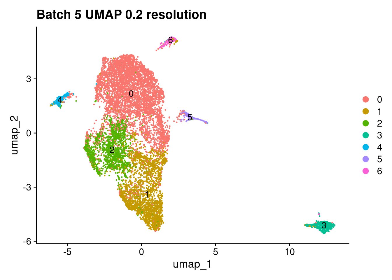
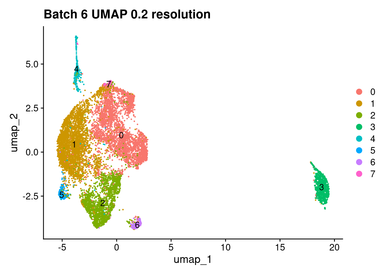
Elapsed time: 1 secondsinvisible(lapply(names(batches), function(nm) {
p <- DimPlot(batches[[nm]], reduction = "umap", label = TRUE) +
ggtitle(glue("Batch {nm} UMAP {res} resolution"))
print(p)
batch_graphs_dir <- file.path(graphs_dir, glue("batch_{nm}"))
ggsave(
filename = file.path(batch_graphs_dir, glue("clusters_batch_{nm}_{res}.pdf")),
plot = p, width = 7, height = 5, dpi = 300, units = "in"
)
}))
for (i in seq_along(batches)) {
  qs_save(batches[[i]], file = paste0(objects_dir, "/batch", i, "_clustered.qs2"))
}files <- list.files(path = objects_dir, pattern = "batch[0-9]+_clustered.qs2", full.names = TRUE)
batches <- lapply(files, qs_read)Gene sets are intersected against the batch feature space before scoring. AddModuleScore calculates average expression of each gene set relative to a randomly sampled control set, giving a background-corrected enrichment score per cell.
myeloid_seu <- intersect(gs_myeloid, rownames(batches[[1]]))
prolif_seu <- intersect(gs_proliferating, rownames(batches[[1]]))
macrophage_seu <- intersect(gs_macrophage, rownames(batches[[1]]))
dendritic_seu <- intersect(gs_dendritic, rownames(batches[[1]]))
gene_sets <- list(
dendritic = dendritic_seu,
proliferating = prolif_seu,
macrophage = macrophage_seu,
myeloid = myeloid_seu,
CRM = gs_crm,
DAM = gs_dam,
HLA = gs_hla,
HM = gs_hm,
IRM = gs_irm,
RM = gs_rm,
tCRM = gs_tcrm
)
batches <- lapply(seq_along(batches), function(i) {
o <- batches[[i]]
nm <- as.character(i)
message(glue("Processing Batch {nm}..."))
batch_graphs_dir <- file.path(graphs_dir, glue("batch_{nm}"))
if (!dir.exists(batch_graphs_dir)) dir.create(batch_graphs_dir, recursive = TRUE)
o <- AddModuleScore(object = o, features = gene_sets, name = names(gene_sets), ctrl = 5, seed = 42)
o$seurat_clusters <- factor(
o$seurat_clusters,
levels = sort(as.numeric(unique(as.character(o$seurat_clusters))))
)
Idents(o) <- "seurat_clusters"
p1 <- VlnPlot(o, features = c("dendritic1", "proliferating2", "macrophage3", "myeloid4"),
group.by = "seurat_clusters", pt.size = 0, ncol = 2) +
ggtitle(glue("Batch {nm}: Cell Types"))
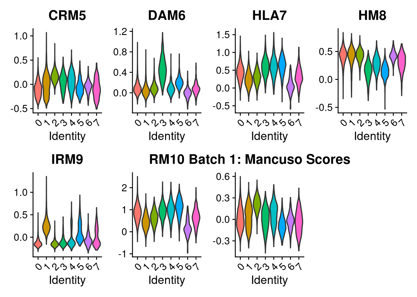
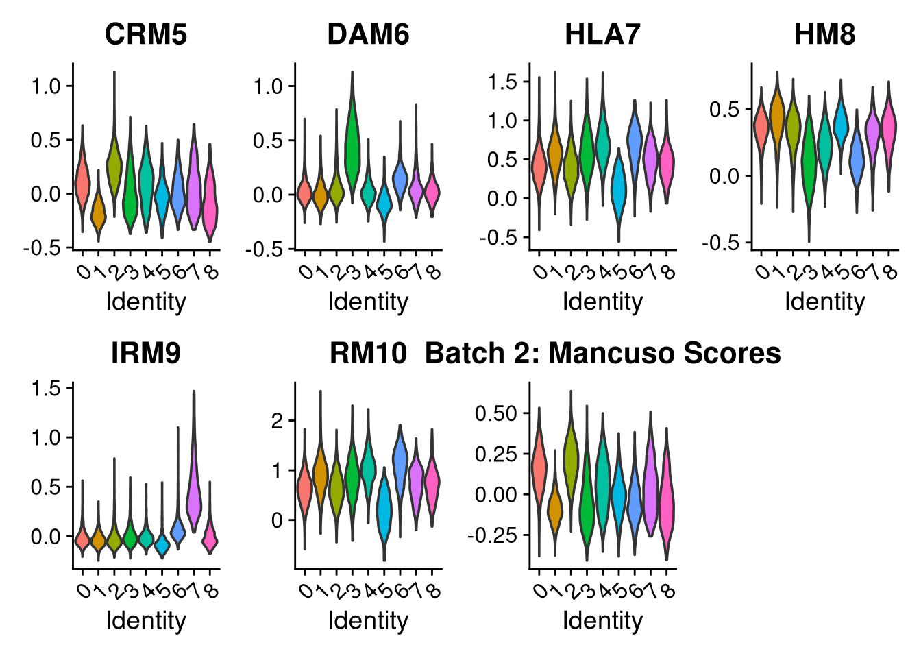
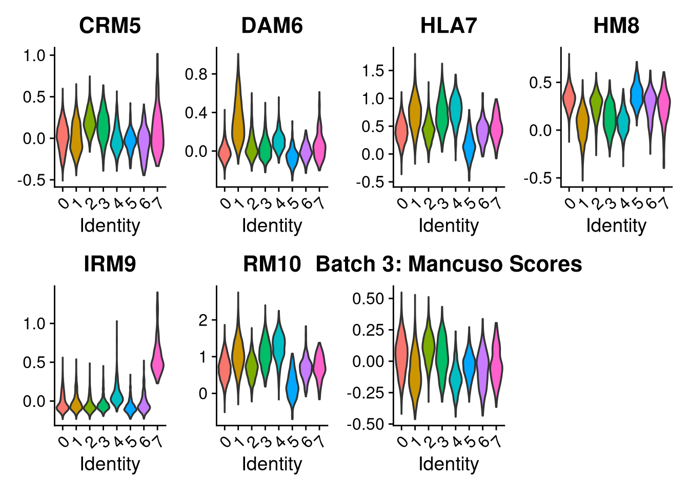
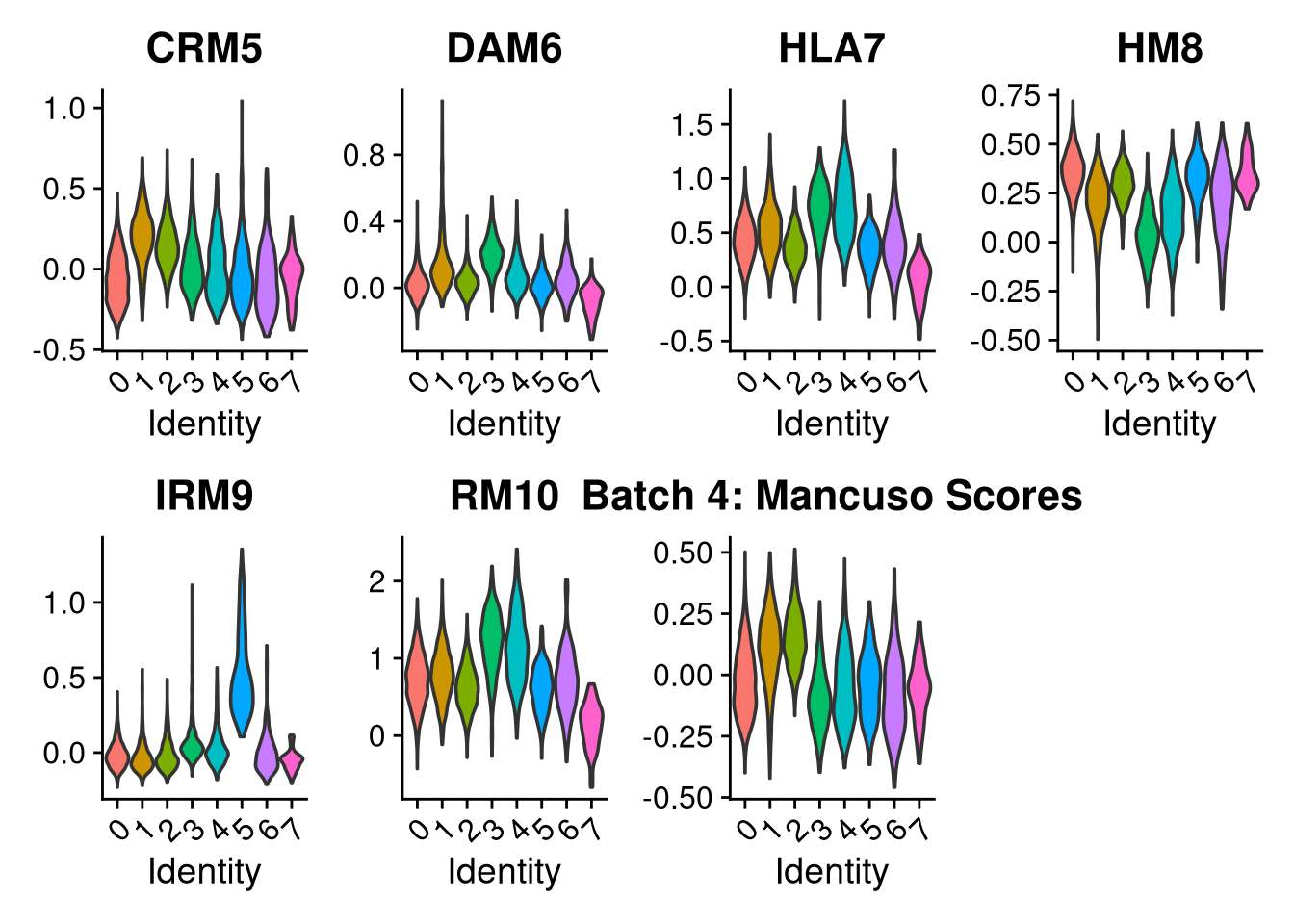
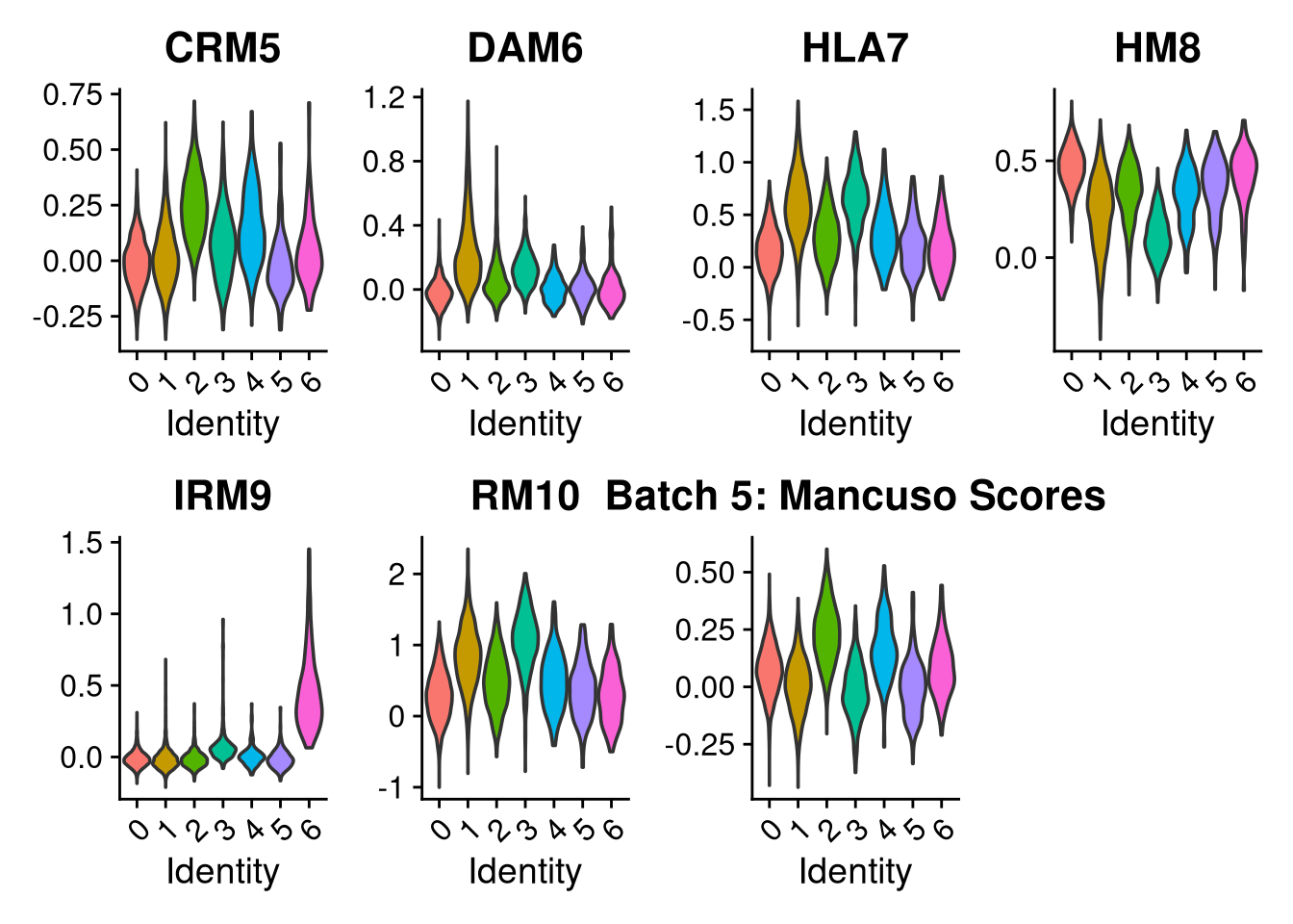
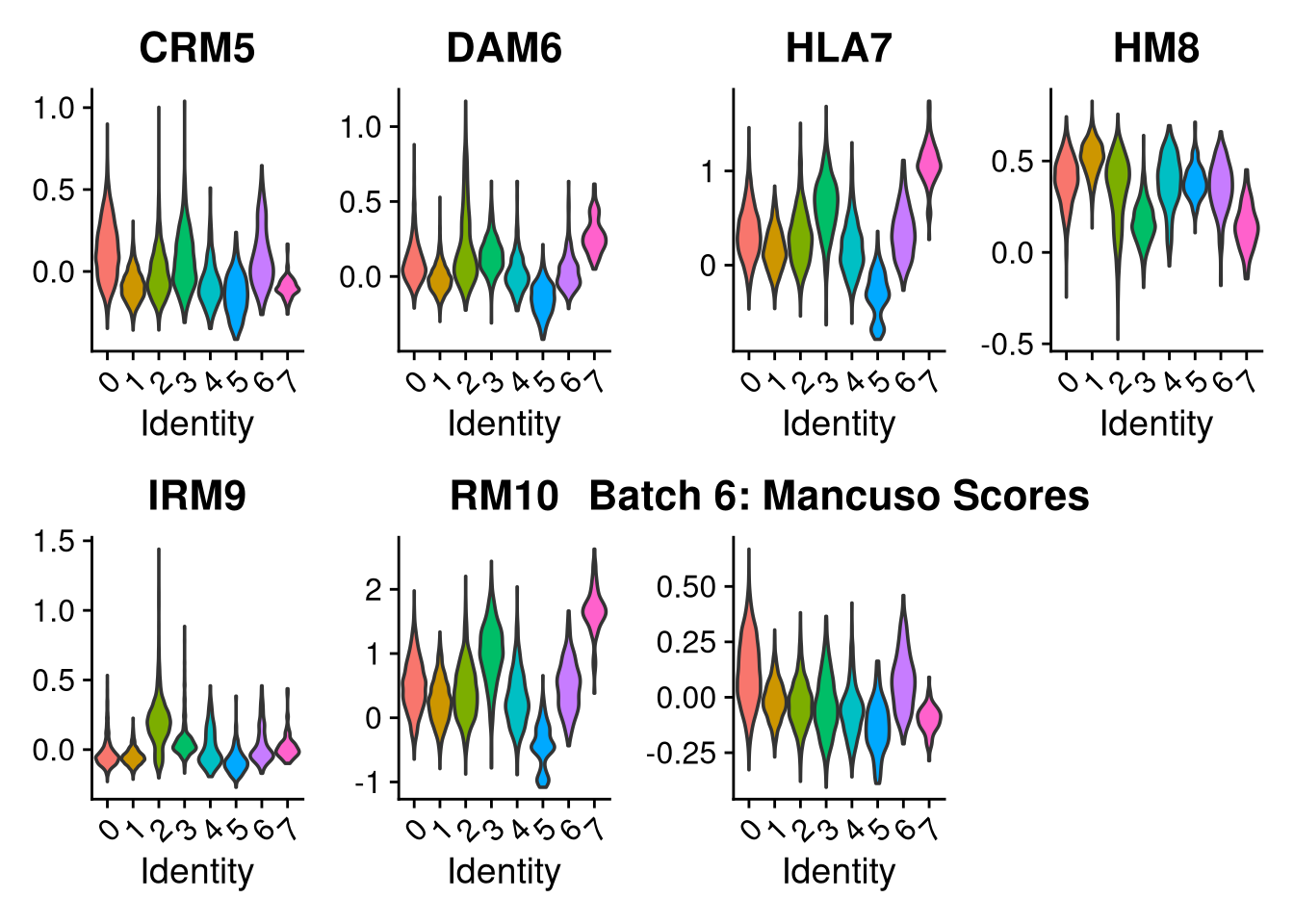
p2 <- VlnPlot(o, features = c("CRM5", "DAM6", "HLA7", "HM8", "IRM9", "RM10", "tCRM11"),
group.by = "seurat_clusters", pt.size = 0, ncol = 4) +
ggtitle(glue("Batch {nm}: Mancuso Scores"))
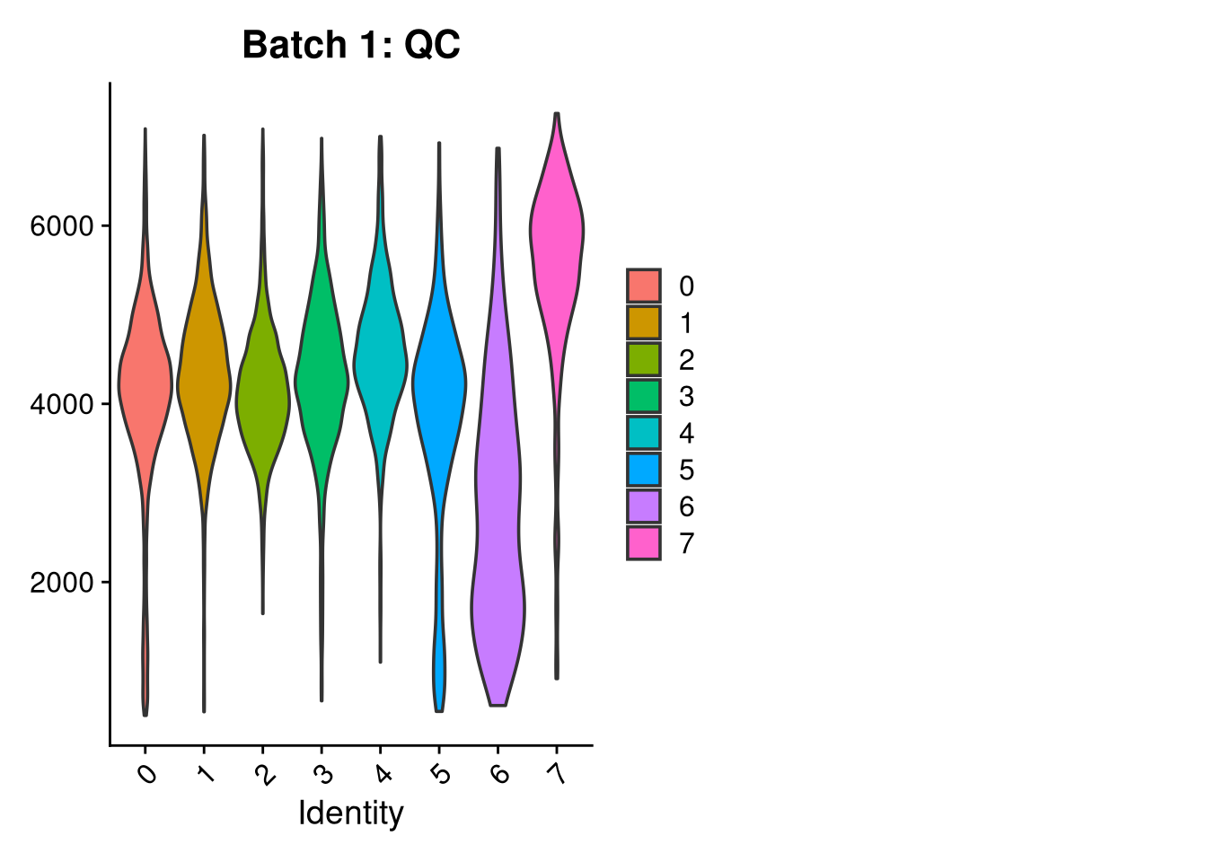
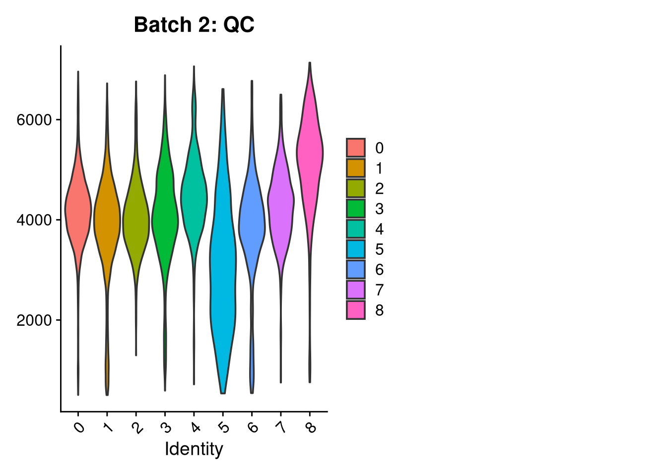
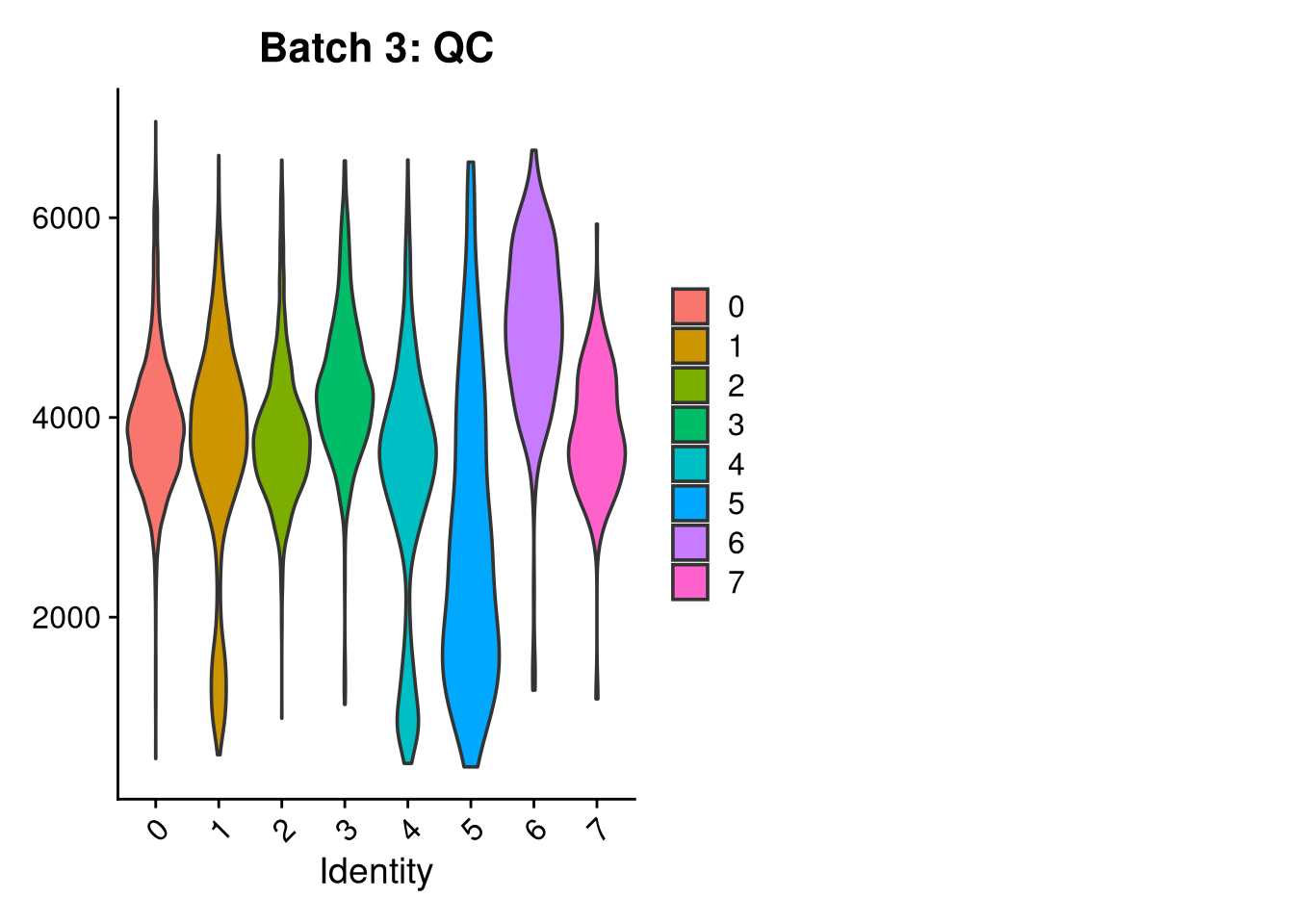
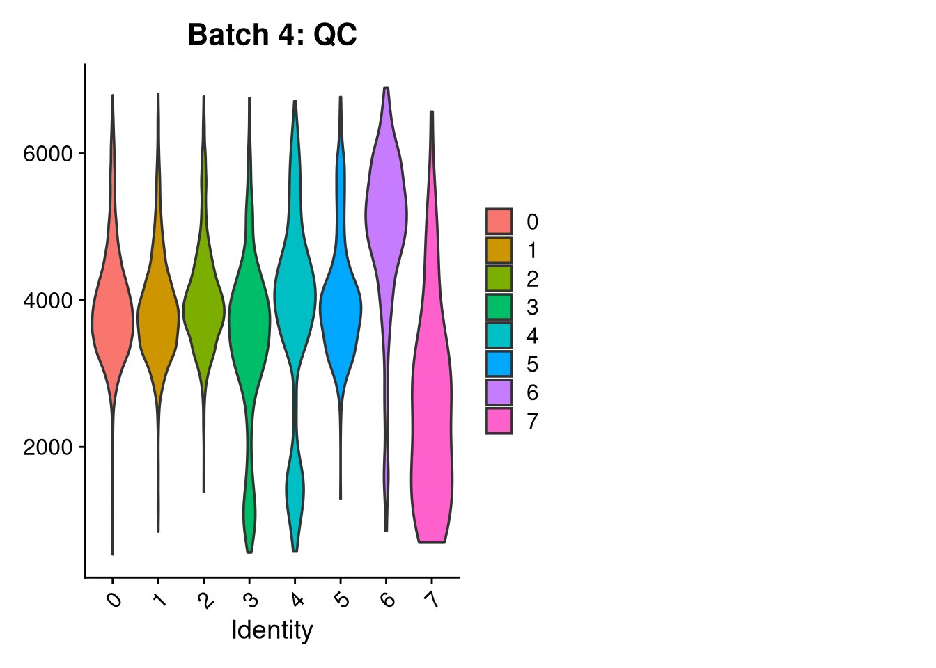
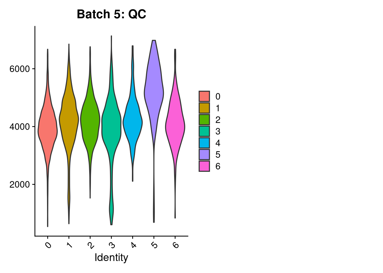
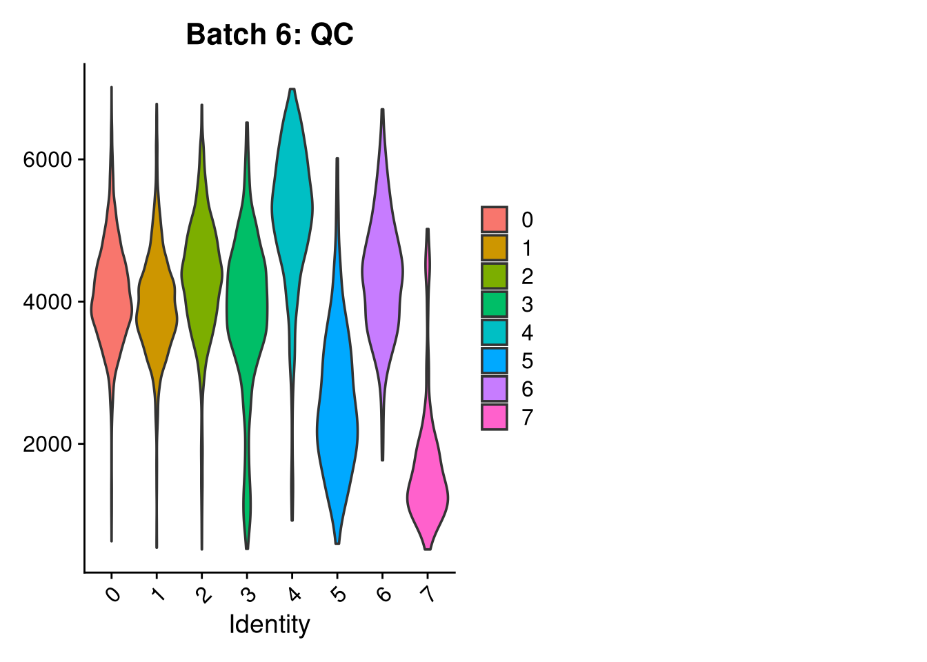
p3 <- VlnPlot(o, features = c("nFeature_RNA"),
group.by = "seurat_clusters", pt.size = 0, ncol = 2) +
ggtitle(glue("Batch {nm}: QC"))
print(p1); print(p2); print(p3)
ggsave(filename = file.path(batch_graphs_dir, glue("batch_{nm}_celltypes.pdf")), plot = p1, width = 7, height = 5, dpi = 300)
ggsave(filename = file.path(batch_graphs_dir, glue("batch_{nm}_mancuso.pdf")), plot = p2, width = 10, height = 5, dpi = 300)
ggsave(filename = file.path(batch_graphs_dir, glue("batch_{nm}_qc.pdf")), plot = p3, width = 10, height = 5, dpi = 300)
return(o)
})Processing Batch 1...Warning: The following features are not present in the object: CCL3L1, IL8,
MIR142, CCL4L1, LINC00936, H3F3B, RN7SL1, SNORD3B-2, AC006129.4, RP11-386I14.4,
MIR24-2, not searching for symbol synonymsWarning: The following features are not present in the object: MT-RNR2,
RP11-536O18.2, FAM129A, AC004086.1, MT-RNR1, C9orf16, TMEM251, ATP5E, PPAP2A,
not searching for symbol synonymsWarning: The following features are not present in the object: GNB2L1, GLTSCR2,
ATP5G2, RPS4Y1, not searching for symbol synonymsWarning: The following features are not present in the object: C1orf63,
FAM105A, GPR56, C10orf54, TMEM173, FYB, RP11-480C22.1, RP11-343N15.5, KIAA1551,
RP1-249H1.4, RP11-439A17.7, not searching for symbol synonymsWarning: The following features are not present in the object: DDX58, FAM26F,
C19orf66, WARS, not searching for symbol synonymsWarning: The following features are not present in the object: GNB2L1, not
searching for symbol synonymsWarning: The following features are not present in the object: LINC00936,
H3F3B, SNORD3B-1, CTA-29F11-1, SNORD3B-2, MT-RNR2, AC253572-2, AC103591-3,
AC020916-1, RP11-386I14-4, MT-RNR1, HIST2H2AA3, MTCO1P12, AP003481-1,
AC004687-1, SNORD3A, AC243960-1, HIST1H4E, RP1-18D14-7, AC245014-3, AL499604-1,
AL118516-1, AL021155-2, HIST1H4C, GGTA1P, RNU2-63P, not searching for symbol
synonyms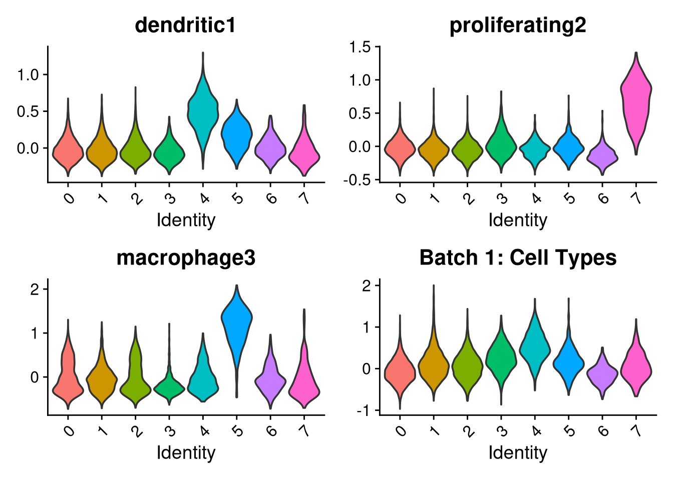
Processing Batch 2...Warning: The following features are not present in the object: CCL3L1, IL8,
MIR142, CCL4L1, LINC00936, H3F3B, RN7SL1, SNORD3B-2, AC006129.4, RP11-386I14.4,
MIR24-2, not searching for symbol synonymsWarning: The following features are not present in the object: MT-RNR2,
RP11-536O18.2, FAM129A, AC004086.1, MT-RNR1, C9orf16, TMEM251, ATP5E, PPAP2A,
not searching for symbol synonymsWarning: The following features are not present in the object: GNB2L1, GLTSCR2,
ATP5G2, RPS4Y1, not searching for symbol synonymsWarning: The following features are not present in the object: C1orf63,
FAM105A, GPR56, C10orf54, TMEM173, FYB, RP11-480C22.1, RP11-343N15.5, KIAA1551,
RP1-249H1.4, RP11-439A17.7, not searching for symbol synonymsWarning: The following features are not present in the object: DDX58, FAM26F,
C19orf66, WARS, not searching for symbol synonymsWarning: The following features are not present in the object: GNB2L1, not
searching for symbol synonymsWarning: The following features are not present in the object: LINC00936,
H3F3B, SNORD3B-1, CTA-29F11-1, SNORD3B-2, MT-RNR2, AC253572-2, AC103591-3,
AC020916-1, RP11-386I14-4, MT-RNR1, HIST2H2AA3, MTCO1P12, AP003481-1,
AC004687-1, SNORD3A, AC243960-1, HIST1H4E, RP1-18D14-7, AC245014-3, AL499604-1,
AL118516-1, AL021155-2, HIST1H4C, GGTA1P, RNU2-63P, not searching for symbol
synonyms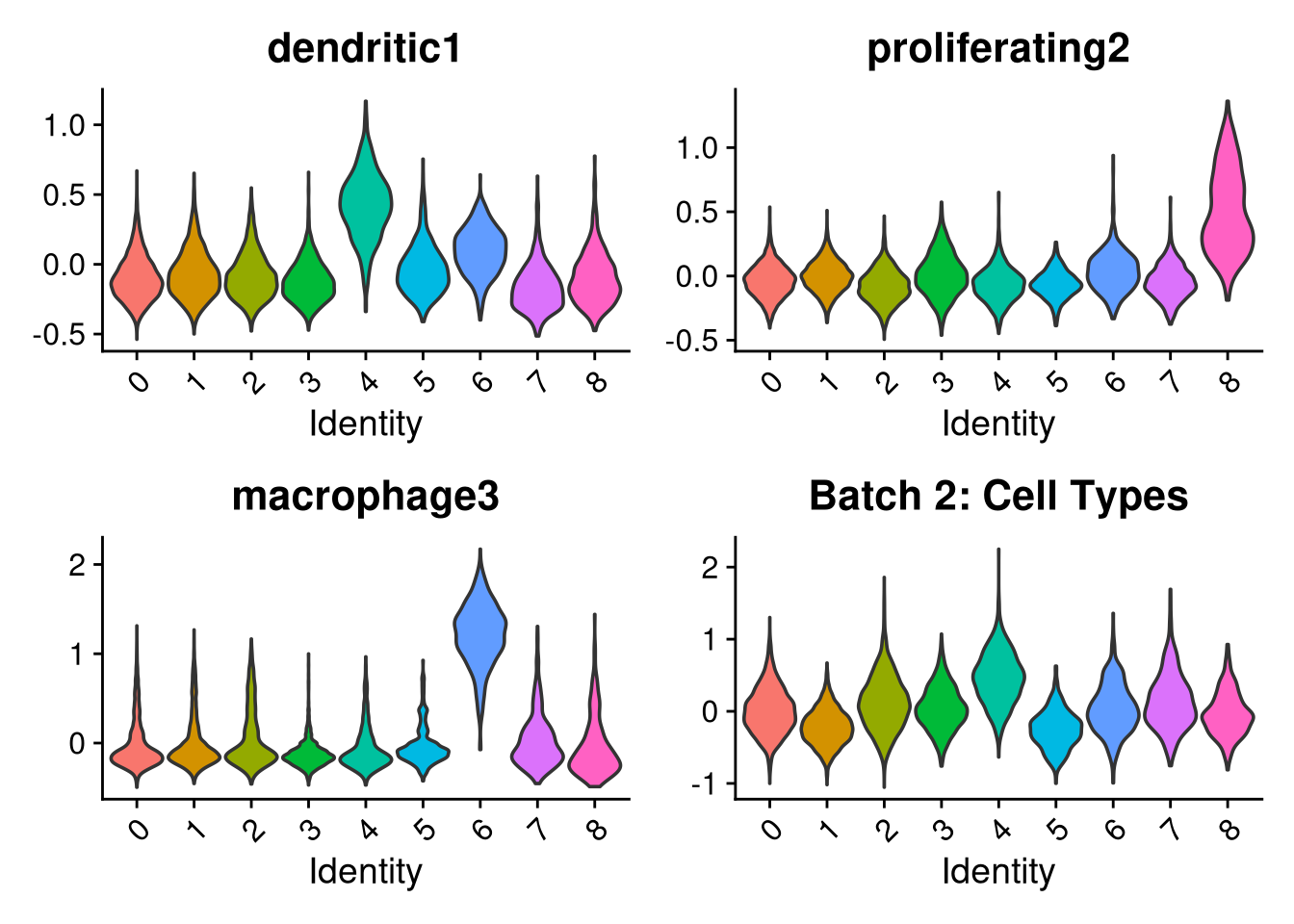
Processing Batch 3...Warning: The following features are not present in the object: CCL3L1, IL8,
MIR142, CCL4L1, LINC00936, H3F3B, RN7SL1, SNORD3B-2, AC006129.4, RP11-386I14.4,
MIR24-2, not searching for symbol synonymsWarning: The following features are not present in the object: MT-RNR2,
RP11-536O18.2, FAM129A, AC004086.1, MT-RNR1, C9orf16, TMEM251, ATP5E, PPAP2A,
not searching for symbol synonymsWarning: The following features are not present in the object: GNB2L1, GLTSCR2,
ATP5G2, RPS4Y1, not searching for symbol synonymsWarning: The following features are not present in the object: C1orf63,
FAM105A, GPR56, C10orf54, TMEM173, FYB, RP11-480C22.1, RP11-343N15.5, KIAA1551,
RP1-249H1.4, RP11-439A17.7, not searching for symbol synonymsWarning: The following features are not present in the object: DDX58, FAM26F,
C19orf66, WARS, not searching for symbol synonymsWarning: The following features are not present in the object: GNB2L1, not
searching for symbol synonymsWarning: The following features are not present in the object: LINC00936,
H3F3B, SNORD3B-1, CTA-29F11-1, SNORD3B-2, MT-RNR2, AC253572-2, AC103591-3,
AC020916-1, RP11-386I14-4, MT-RNR1, HIST2H2AA3, MTCO1P12, AP003481-1,
AC004687-1, SNORD3A, AC243960-1, HIST1H4E, RP1-18D14-7, AC245014-3, AL499604-1,
AL118516-1, AL021155-2, HIST1H4C, GGTA1P, RNU2-63P, not searching for symbol
synonyms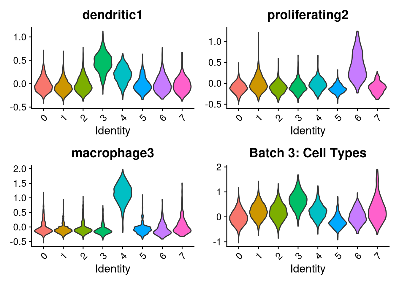
Processing Batch 4...Warning: The following features are not present in the object: CCL3L1, IL8,
MIR142, CCL4L1, LINC00936, H3F3B, RN7SL1, SNORD3B-2, AC006129.4, RP11-386I14.4,
MIR24-2, not searching for symbol synonymsWarning: The following features are not present in the object: MT-RNR2,
RP11-536O18.2, FAM129A, AC004086.1, MT-RNR1, C9orf16, TMEM251, ATP5E, PPAP2A,
not searching for symbol synonymsWarning: The following features are not present in the object: GNB2L1, GLTSCR2,
ATP5G2, RPS4Y1, not searching for symbol synonymsWarning: The following features are not present in the object: C1orf63,
FAM105A, GPR56, C10orf54, TMEM173, FYB, RP11-480C22.1, RP11-343N15.5, KIAA1551,
RP1-249H1.4, RP11-439A17.7, not searching for symbol synonymsWarning: The following features are not present in the object: DDX58, FAM26F,
C19orf66, WARS, TNFAIP6, not searching for symbol synonymsWarning: The following features are not present in the object: GNB2L1, not
searching for symbol synonymsWarning: The following features are not present in the object: LINC00936,
H3F3B, SNORD3B-1, CTA-29F11-1, SNORD3B-2, MT-RNR2, AC253572-2, AC103591-3,
AC020916-1, RP11-386I14-4, MT-RNR1, HIST2H2AA3, MTCO1P12, AP003481-1,
AC004687-1, SNORD3A, AC243960-1, HIST1H4E, RP1-18D14-7, AC245014-3, AL499604-1,
AL118516-1, AL021155-2, HIST1H4C, GGTA1P, RNU2-63P, not searching for symbol
synonyms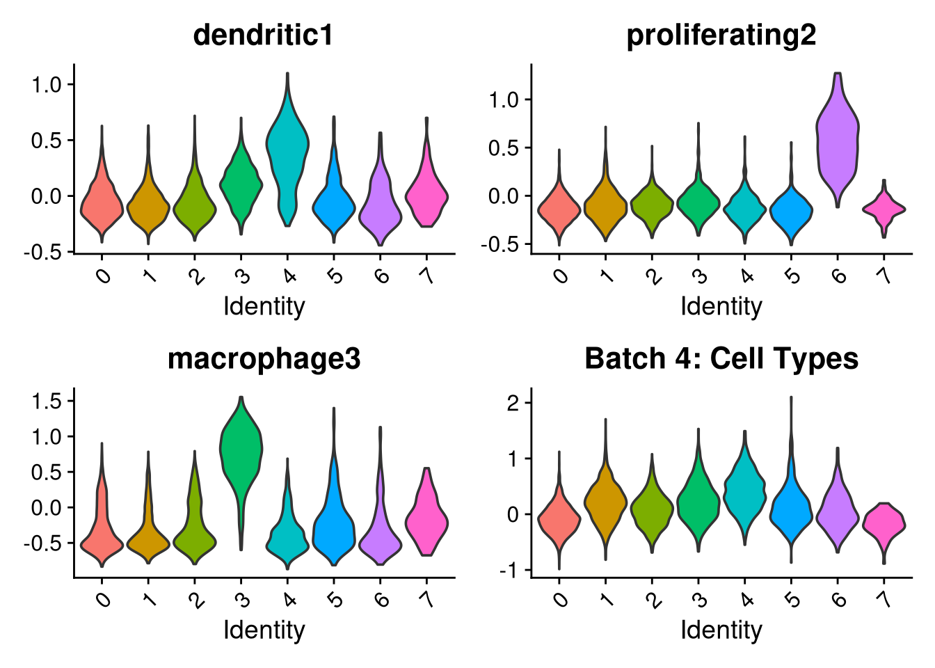
Processing Batch 5...Warning: The following features are not present in the object: CCL3L1, IL8,
MIR142, CCL4L1, LINC00936, H3F3B, RN7SL1, SNORD3B-2, AC006129.4, RP11-386I14.4,
MIR24-2, not searching for symbol synonymsWarning: The following features are not present in the object: MT-RNR2,
RP11-536O18.2, FAM129A, AC004086.1, MT-RNR1, C9orf16, TMEM251, ATP5E, PPAP2A,
not searching for symbol synonymsWarning: The following features are not present in the object: GNB2L1, GLTSCR2,
ATP5G2, RPS4Y1, not searching for symbol synonymsWarning: The following features are not present in the object: C1orf63,
FAM105A, GPR56, C10orf54, TMEM173, FYB, RP11-480C22.1, RP11-343N15.5, KIAA1551,
RP1-249H1.4, RP11-439A17.7, not searching for symbol synonymsWarning: The following features are not present in the object: DDX58, FAM26F,
C19orf66, WARS, TNFAIP6, CXCL11, not searching for symbol synonymsWarning: The following features are not present in the object: GNB2L1, not
searching for symbol synonymsWarning: The following features are not present in the object: LINC00936,
H3F3B, SNORD3B-1, CTA-29F11-1, SNORD3B-2, MT-RNR2, AC253572-2, AC103591-3,
AC020916-1, RP11-386I14-4, MT-RNR1, HIST2H2AA3, MTCO1P12, AP003481-1,
AC004687-1, SNORD3A, AC243960-1, HIST1H4E, RP1-18D14-7, AC245014-3, AL499604-1,
AL118516-1, AL021155-2, HIST1H4C, GGTA1P, RNU2-63P, not searching for symbol
synonyms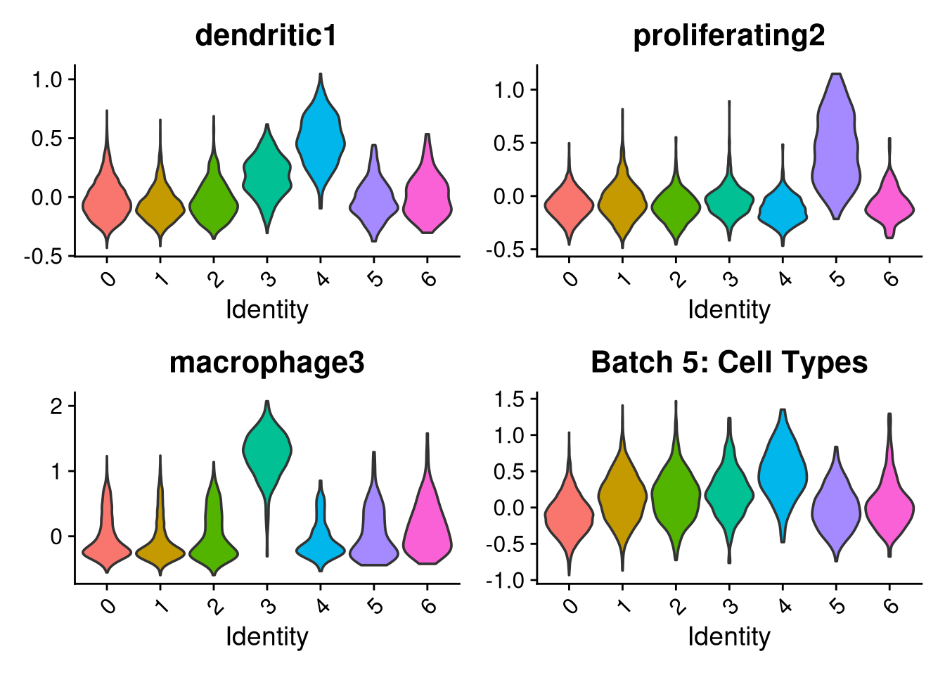
Processing Batch 6...Warning: The following features are not present in the object: CCL3L1, IL8,
MIR142, CCL4L1, LINC00936, H3F3B, RN7SL1, SNORD3B-2, AC006129.4, RP11-386I14.4,
MIR24-2, not searching for symbol synonymsWarning: The following features are not present in the object: MT-RNR2,
RP11-536O18.2, FAM129A, AC004086.1, MT-RNR1, C9orf16, TMEM251, ATP5E, PPAP2A,
not searching for symbol synonymsWarning: The following features are not present in the object: GNB2L1, GLTSCR2,
ATP5G2, RPS4Y1, not searching for symbol synonymsWarning: The following features are not present in the object: C1orf63,
FAM105A, GPR56, C10orf54, TMEM173, FYB, RP11-480C22.1, RP11-343N15.5, KIAA1551,
RP1-249H1.4, RP11-439A17.7, not searching for symbol synonymsWarning: The following features are not present in the object: DDX58, FAM26F,
C19orf66, WARS, TNFAIP6, CXCL11, not searching for symbol synonymsWarning: The following features are not present in the object: GNB2L1, not
searching for symbol synonymsWarning: The following features are not present in the object: LINC00936,
H3F3B, SNORD3B-1, CTA-29F11-1, SNORD3B-2, MT-RNR2, AC253572-2, AC103591-3,
AC020916-1, RP11-386I14-4, MT-RNR1, HIST2H2AA3, MTCO1P12, AP003481-1,
AC004687-1, SNORD3A, AC243960-1, HIST1H4E, RP1-18D14-7, AC245014-3, AL499604-1,
AL118516-1, AL021155-2, HIST1H4C, GGTA1P, RNU2-63P, not searching for symbol
synonyms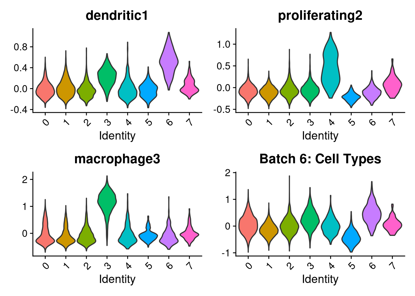
Batches are merged back into a single object and re-normalised with SCTransform v2. PCA is then run on the merged, unintegrated object to provide the input embedding required by RPCA. Integration with IntegrateLayers (RPCA method) corrects pool-level batch effects while aiming to preserve biological variance.
merged_obj <- merge(batches[[1]], y = batches[-1])
Idents(merged_obj) <- "pool_id"

options(future.globals.maxSize = 100 * 1024^3)
merged_obj <- SCTransform(merged_obj, vst.flavor = "v2", verbose = FALSE)
merged_obj <- RunPCA(merged_obj, verbose = FALSE, assay = "SCT")

set.seed(42)
int_method <- "rpca"
DefaultAssay(merged_obj) <- "SCT"
merged_obj <- IntegrateLayers(
  object               = merged_obj,
  method               = RPCAIntegration,
  normalization.method = "SCT",
  orig.reduction       = "pca",
  new.reduction        = glue("integrated.{int_method}"),
  verbose              = FALSE
)
Warning: UNRELIABLE VALUE: One of the 'future.apply' iterations
('future_lapply-1') unexpectedly generated random numbers without declaring so.
There is a risk that those random numbers are not statistically sound and the
overall results might be invalid. To fix this, specify 'future.seed=TRUE'. This
ensures that proper, parallel-safe random numbers are produced via a parallel
RNG method. To disable this check, use 'future.seed = NULL', or set option
'future.rng.onMisuse' to "ignore". [future 'future_lapply-1'
(8be034ec696f25278ad3a140970bf912-59); on
8be034ec696f25278ad3a140970bf912@cn027<902421>]Neighbours are found on the integrated RPCA reduction and clusters are identified at resolution 0.2. A UMAP is computed on the same integrated reduction for visualisation.
set.seed(42)
merged_obj <- FindNeighbors(merged_obj, reduction = glue("integrated.{int_method}"), dims = 1:30)
Computing nearest neighbor graphComputing SNNset.seed(42)
cluster_resolution <- 0.2
merged_obj <- FindClusters(
merged_obj,
resolution = cluster_resolution,
cluster.name = glue("{int_method}_clusters"),
graph.name = "SCT_snn"
)Modularity Optimizer version 1.3.0 by Ludo Waltman and Nees Jan van Eck
Number of nodes: 86504
Number of edges: 2726533
Running Louvain algorithm...
Maximum modularity in 10 random starts: 0.9195
Number of communities: 12
Elapsed time: 52 secondsset.seed(42)
merged_obj <- RunUMAP(
merged_obj,
dims = 1:30,
reduction.name = glue("umap.{int_method}")
)18:18:58 UMAP embedding parameters a = 0.9922 b = 1.11218:18:58 Read 86504 rows and found 30 numeric columns18:18:58 Using Annoy for neighbor search, n_neighbors = 3018:18:58 Building Annoy index with metric = cosine, n_trees = 500% 10 20 30 40 50 60 70 80 90 100%[----|----|----|----|----|----|----|----|----|----|**************************************************|
18:19:04 Writing NN index file to temp file /tmp/slurm_45934587/RtmpfBZYPK/filedc515768aef1f
18:19:05 Searching Annoy index using 1 thread, search_k = 3000
18:19:35 Annoy recall = 100%
18:19:37 Commencing smooth kNN distance calibration using 1 thread with target n_neighbors = 30
18:19:43 Initializing from normalized Laplacian + noise (using RSpectra)
18:19:47 Commencing optimization for 200 epochs, with 3937638 positive edges
18:19:47 Using rng type: pcg
18:20:27 Optimization finishedqs_save(merged_obj, file = file.path(objects_dir, "prelabelled_integrated_rpca.qs2"))
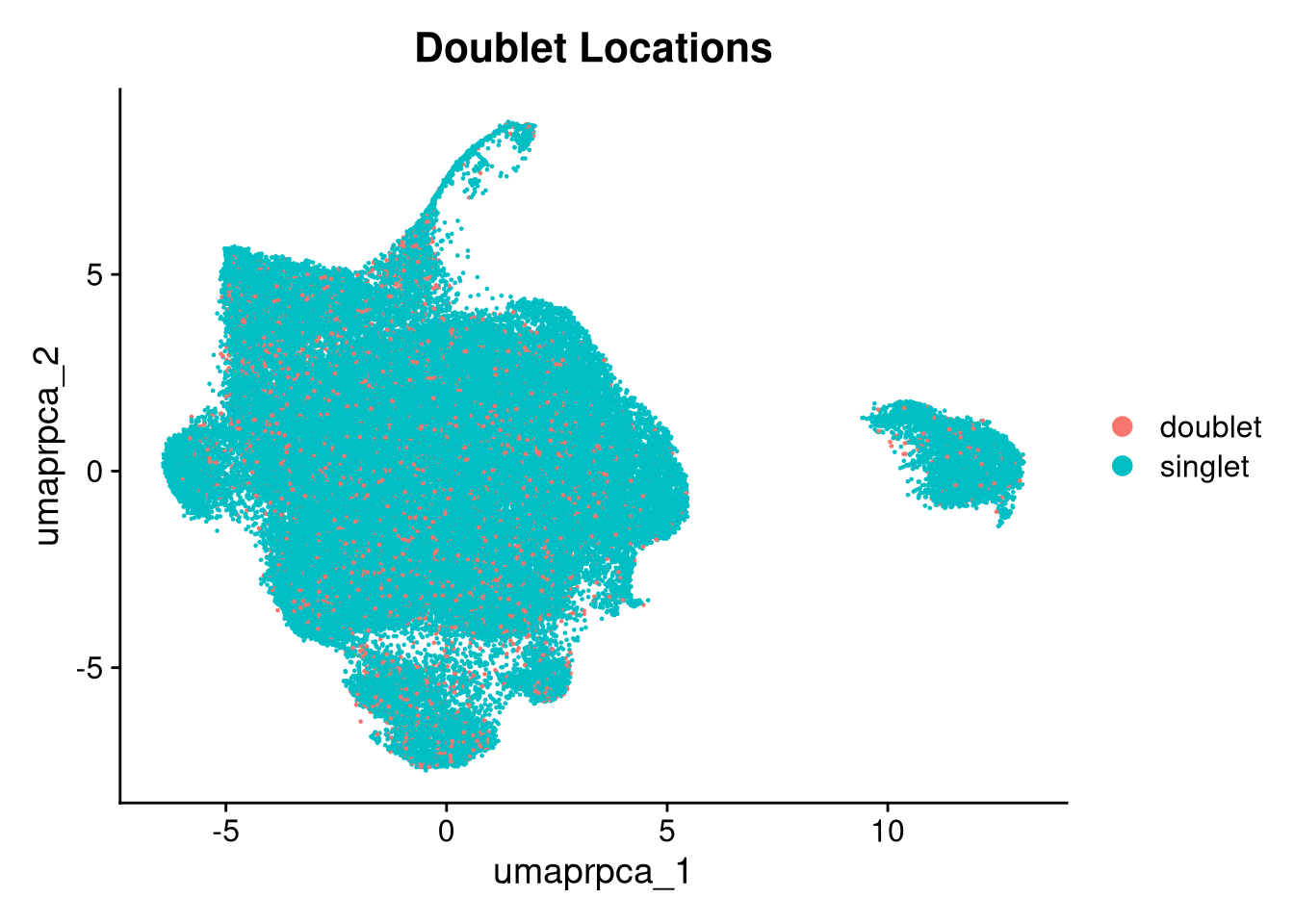
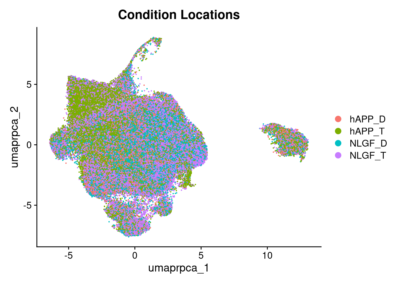
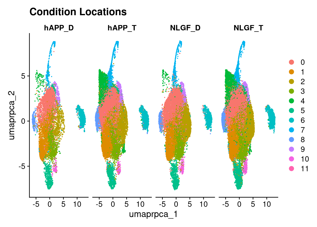
merged_obj <- qs_read(file.path(objects_dir, "prelabelled_integrated_rpca.qs2"))A standard set of diagnostic plots checks cluster structure, sample and pool mixing, QC metric distributions, doublet and outlier locations, and condition separation.
p1 <- DimPlot(merged_obj, reduction = glue("umap.{int_method}"),
group.by = glue("{int_method}_clusters"), label = TRUE) +
ggtitle(glue("Clusters {cluster_resolution} resolution"))
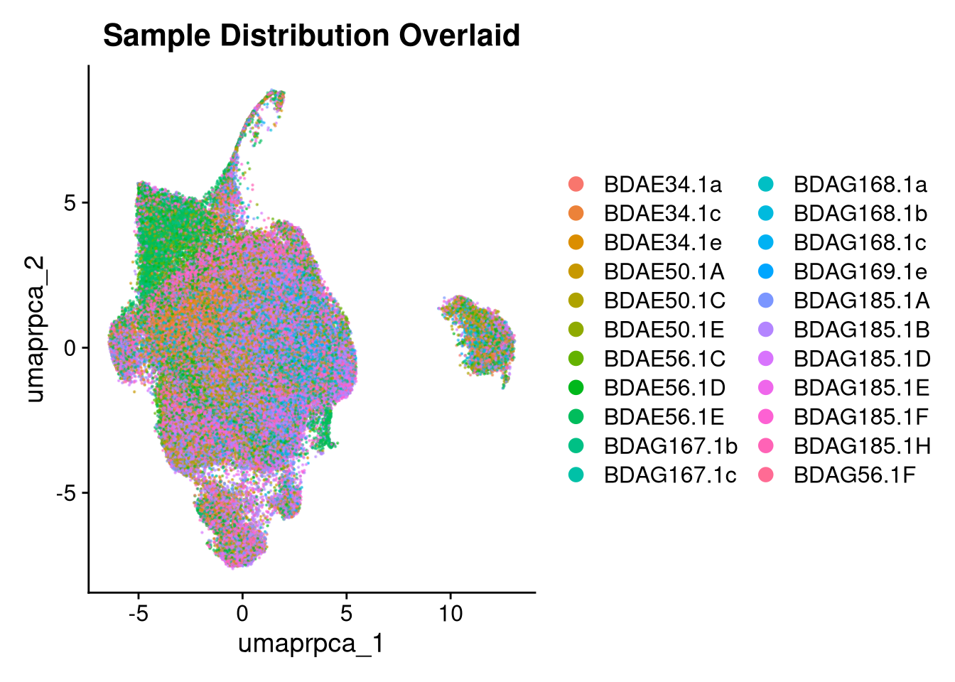
p2 <- DimPlot(merged_obj, reduction = glue("umap.{int_method}"),
group.by = "orig.ident", shuffle = TRUE, alpha = 0.5) +
ggtitle("Sample Distribution Overlaid")
p2.5 <- DimPlot(merged_obj, reduction = glue("umap.{int_method}"),
split.by = "orig.ident", ncol = 5, alpha = 0.5) +
ggtitle("Sample Distribution Split")
p3 <- DimPlot(merged_obj, reduction = glue("umap.{int_method}"),
group.by = "pool_id", shuffle = TRUE, alpha = 0.5) +
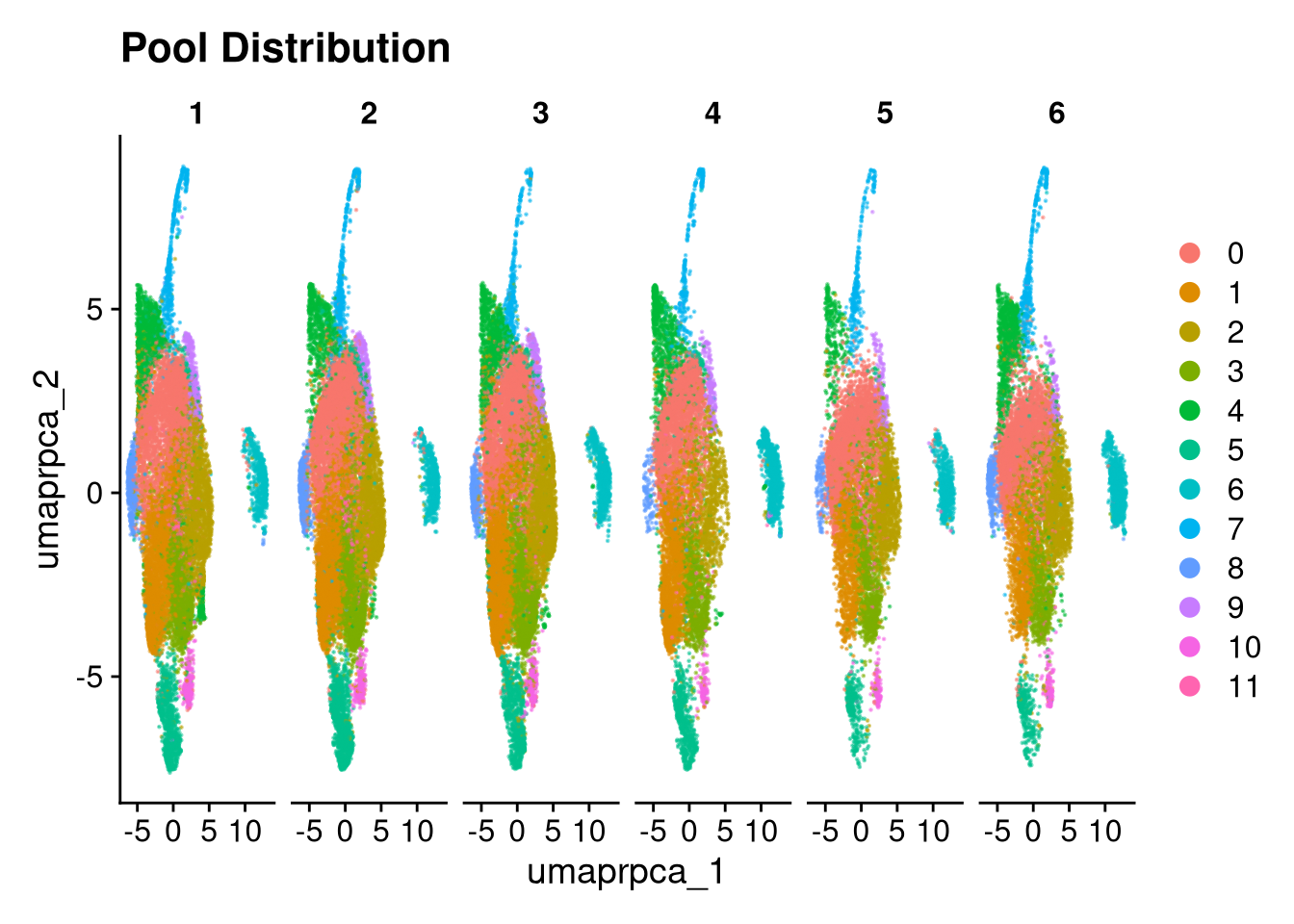
ggtitle("Pool Distribution")
p3.5 <- DimPlot(merged_obj, reduction = glue("umap.{int_method}"),
split.by = "pool_id", shuffle = TRUE, alpha = 0.5) +
ggtitle("Pool Distribution")
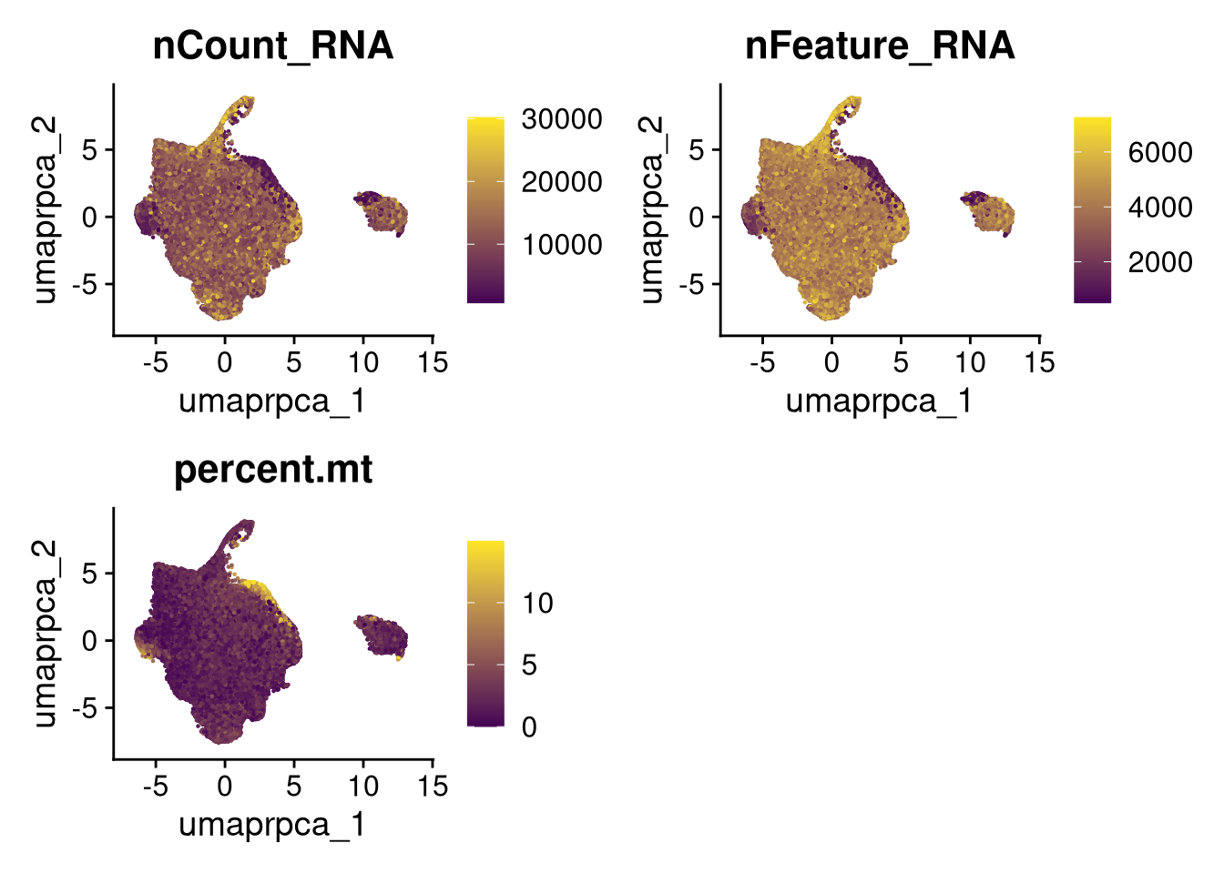
p4 <- FeaturePlot(merged_obj, reduction = glue("umap.{int_method}"),
features = c("nCount_RNA", "nFeature_RNA", "percent.mt"),
cols = c("#440154", "#FDE725"))
p5 <- DimPlot(merged_obj, reduction = glue("umap.{int_method}"),
group.by = "scDblFinder.class") +
ggtitle("Doublet Locations")
p5.5 <- DimPlot(merged_obj, reduction = glue("umap.{int_method}"),
group.by = "mad3_outlier") +
ggtitle("MAD3 Outlier Locations")
p6 <- DimPlot(merged_obj, reduction = glue("umap.{int_method}"),
group.by = "group_id", shuffle = TRUE) +
ggtitle("Condition Locations")
p6.5 <- DimPlot(merged_obj, reduction = glue("umap.{int_method}"),
split.by = "group_id", ncol = 5) +
ggtitle("Condition Locations")
print(p1); print(p2); print(p2.5)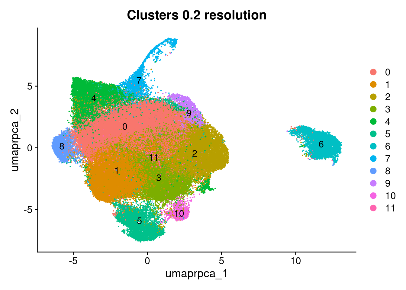

print(p3); print(p4); print(p5)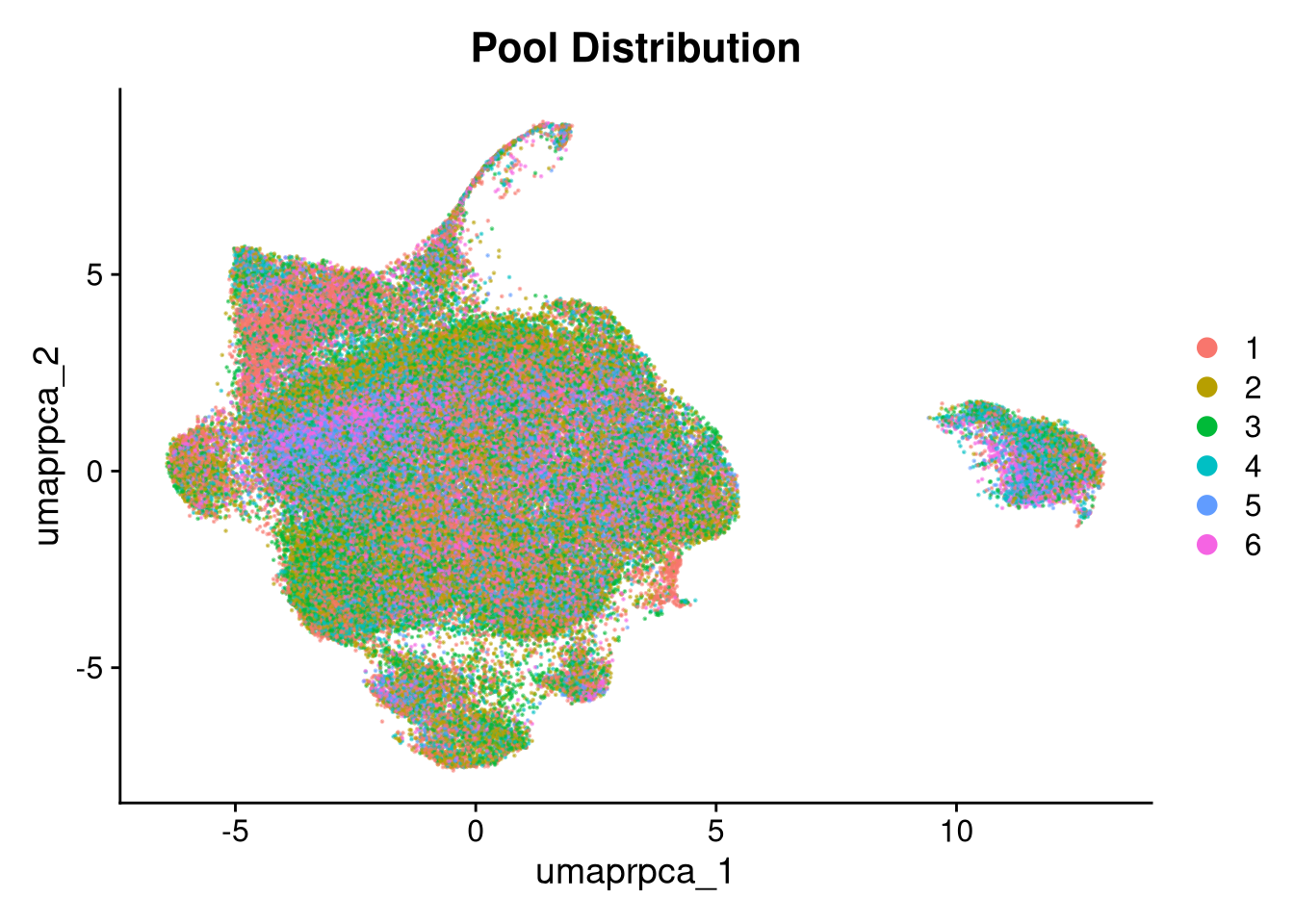
print(p5.5); print(p6); print(p6.5); print(p3.5)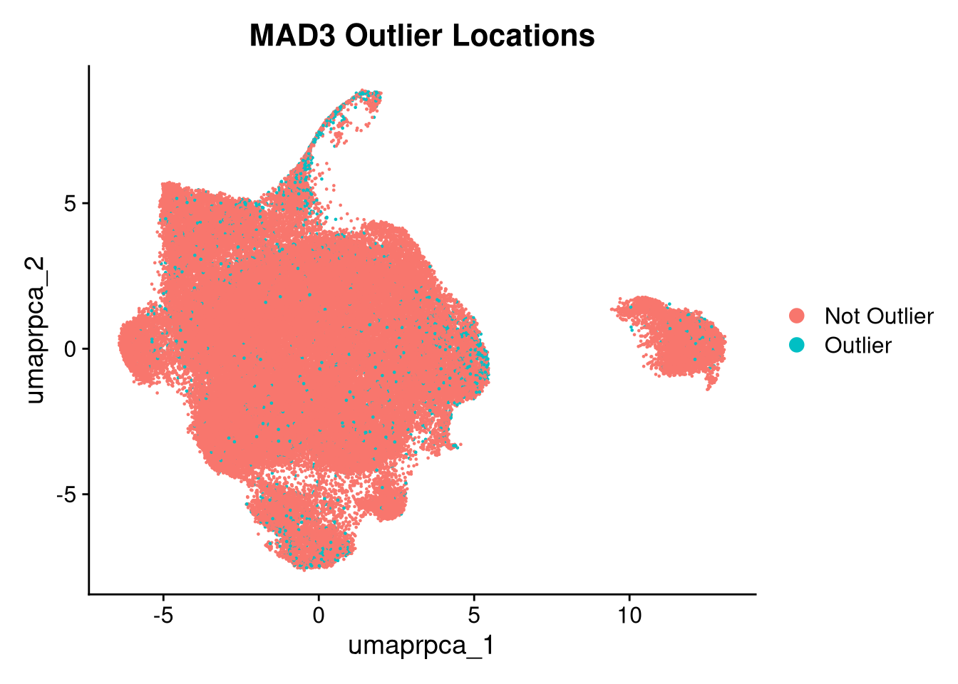
ggsave(filename = file.path(graphs_dir, int_method, cluster_resolution, glue("integrated_{int_method}_clusters_{cluster_resolution}.pdf")),       plot = p1,   width = 7,  height = 5, dpi = 300, units = "in")
ggsave(filename = file.path(graphs_dir, int_method, cluster_resolution, glue("integrated_{int_method}_sample_dist_overlaid.pdf")),                plot = p2,   width = 7,  height = 5, dpi = 300, units = "in")
ggsave(filename = file.path(graphs_dir, int_method, cluster_resolution, glue("integrated_{int_method}_sample_dist_split.pdf")),                   plot = p2.5, width = 7,  height = 5, dpi = 300, units = "in")
ggsave(filename = file.path(graphs_dir, int_method, cluster_resolution, glue("integrated_{int_method}_batch_dist.pdf")),                          plot = p3,   width = 7,  height = 5, dpi = 300, units = "in")
ggsave(filename = file.path(graphs_dir, int_method, cluster_resolution, glue("integrated_{int_method}_batch_dist_split.pdf")),                    plot = p3.5, width = 10, height = 5, dpi = 300, units = "in")
ggsave(filename = file.path(graphs_dir, int_method, cluster_resolution, glue("integrated_{int_method}_qc.pdf")),                                  plot = p4,   width = 7,  height = 5, dpi = 300, units = "in")
ggsave(filename = file.path(graphs_dir, int_method, cluster_resolution, glue("integrated_{int_method}_doublet_dist.pdf")),                        plot = p5,   width = 7,  height = 5, dpi = 300, units = "in")
ggsave(filename = file.path(graphs_dir, int_method, cluster_resolution, glue("integrated_{int_method}_outlier_dist.pdf")),                        plot = p5.5, width = 7,  height = 5, dpi = 300, units = "in")
ggsave(filename = file.path(graphs_dir, int_method, cluster_resolution, glue("integrated_{int_method}_condition_dist_overlaid.pdf")),              plot = p6,   width = 7,  height = 5, dpi = 300, units = "in")
ggsave(filename = file.path(graphs_dir, int_method, cluster_resolution, glue("integrated_{int_method}_condition_dist_split.pdf")), plot = p6.5, width = 7, height = 5, dpi = 300, units = "in")JoinLayers collapses the separate per-pool raw count matrices into a single layer, required for downstream functions. Log-normalisation corrects for differences in sequencing depth, and ScaleData z-scores expression so that highly expressed genes do not dominate dotplots and heatmaps.
DefaultAssay(merged_obj) <- "RNA"
merged_obj <- JoinLayers(merged_obj, assay = "RNA")
merged_obj <- NormalizeData(merged_obj)
Normalizing layer: countsmerged_obj <- ScaleData(merged_obj)Centering and scaling data matrixModule scores are calculated for all Mancuso microglial states and non-microglial cell types on the integrated object. Gene sets are re-intersected here against the merged object feature space. Scores are plotted per cluster to guide annotation.
myeloid_seu    <- intersect(gs_myeloid,       rownames(merged_obj))
prolif_seu     <- intersect(gs_proliferating, rownames(merged_obj))
macrophage_seu <- intersect(gs_macrophage,    rownames(merged_obj))
dendritic_seu  <- intersect(gs_dendritic,     rownames(merged_obj))

gene_sets <- list(
  dendritic     = dendritic_seu,
  proliferating = prolif_seu,
  macrophage    = macrophage_seu,
  myeloid       = myeloid_seu,
  CRM           = gs_crm,
  DAM           = gs_dam,
  HLA           = gs_hla,
  HM            = gs_hm,
  IRM           = gs_irm,
  RM            = gs_rm,
  tCRM          = gs_tcrm
)

merged_obj <- AddModuleScore(merged_obj, features = gene_sets, name = names(gene_sets))
Warning: The following features are not present in the object: CCL3L1, IL8,
MIR142, CCL4L1, LINC00936, H3F3B, RN7SL1, SNORD3B-2, AC006129.4, RP11-386I14.4,
MIR24-2, not searching for symbol synonymsWarning: The following features are not present in the object: MT-RNR2,
RP11-536O18.2, FAM129A, AC004086.1, MT-RNR1, C9orf16, TMEM251, ATP5E, PPAP2A,
not searching for symbol synonymsWarning: The following features are not present in the object: GNB2L1, GLTSCR2,
ATP5G2, not searching for symbol synonymsWarning: The following features are not present in the object: C1orf63,
FAM105A, GPR56, C10orf54, TMEM173, FYB, RP11-480C22.1, RP11-343N15.5, KIAA1551,
RP1-249H1.4, RP11-439A17.7, not searching for symbol synonymsWarning: The following features are not present in the object: DDX58, FAM26F,
C19orf66, WARS, not searching for symbol synonymsWarning: The following features are not present in the object: GNB2L1, not
searching for symbol synonymsWarning: The following features are not present in the object: LINC00936,
H3F3B, SNORD3B-1, CTA-29F11-1, SNORD3B-2, MT-RNR2, AC253572-2, AC103591-3,
AC020916-1, RP11-386I14-4, MT-RNR1, HIST2H2AA3, MTCO1P12, AP003481-1,
AC004687-1, SNORD3A, AC243960-1, HIST1H4E, RP1-18D14-7, AC245014-3, AL499604-1,
AL118516-1, AL021155-2, HIST1H4C, GGTA1P, RNU2-63P, not searching for symbol
synonymsmerged_obj$seurat_clusters <- factor(
merged_obj$rpca_clusters,
levels = sort(as.numeric(unique(as.character(merged_obj$rpca_clusters))))
)
merged_obj$seurat_clusters <- Idents(merged_obj)
p <- VlnPlot(merged_obj, features = c("dendritic1", "proliferating2", "macrophage3", "myeloid4"),
group.by = "seurat_clusters", pt.size = 0, ncol = 2)
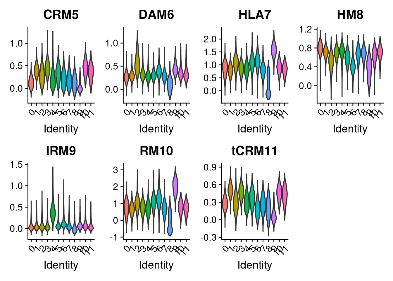
p2 <- VlnPlot(merged_obj, features = c("CRM5", "DAM6", "HLA7", "HM8", "IRM9", "RM10", "tCRM11"),
group.by = "seurat_clusters", pt.size = 0, ncol = 4)
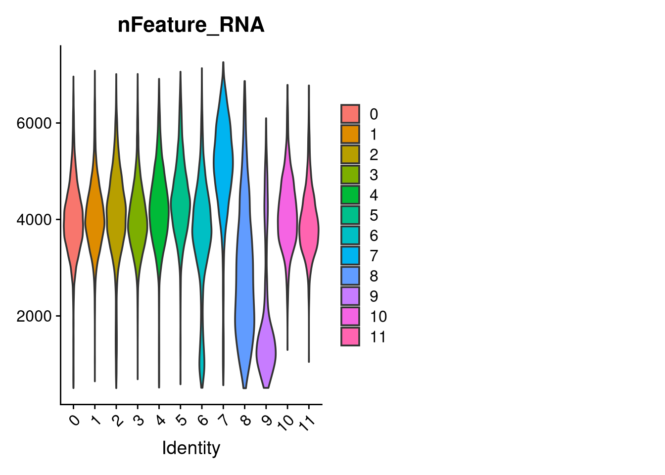
p3 <- VlnPlot(merged_obj, features = c("nFeature_RNA"),
group.by = "seurat_clusters", pt.size = 0, ncol = 2)
ggsave(filename = file.path(graphs_dir, int_method, cluster_resolution, glue("integrated_{int_method}_clusters_vs_nonmicroglia_{cluster_resolution}.pdf")), plot = p, width = 7, height = 5, dpi = 300, units = "in")
ggsave(filename = file.path(graphs_dir, int_method, cluster_resolution, glue("integrated_{int_method}_clusters_vs_mancuso_{cluster_resolution}.pdf")), plot = p2, width = 10, height = 5, dpi = 300, units = "in")
ggsave(filename = file.path(graphs_dir, int_method, cluster_resolution, glue("integrated_{int_method}_clusters_vs_features_{cluster_resolution}.pdf")), plot = p3, width = 10, height = 5, dpi = 300, units = "in")
print(p); print(p2); print(p3)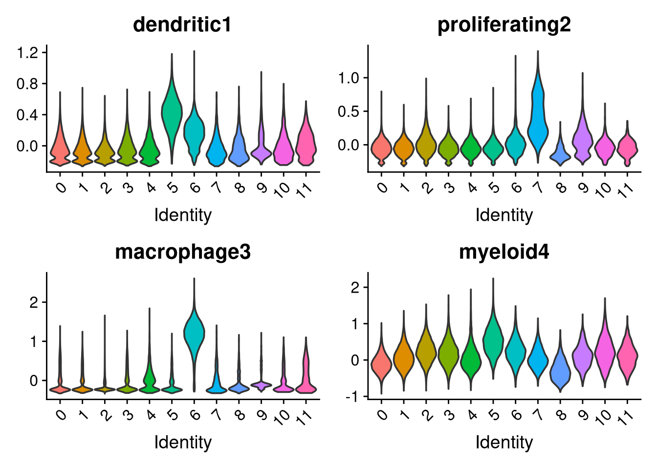
table(merged_obj$seurat_clusters)
    0     1     2     3     4     5     6     7     8     9    10    11
23725 17263 10984 10686 6716 4772 4512 2402 2041 1508 1024 871 Marker genes are identified per cluster using a Wilcoxon rank-sum test. Only positive markers are returned, filtered to a minimum 25% detection rate and log2FC ≥ 0.25. The top 10 markers per cluster by log2FC are printed.
DefaultAssay(merged_obj) <- "RNA"
Idents(merged_obj) <- glue("{int_method}_clusters")
markers <- FindAllMarkers(
  merged_obj,
  test.use      = "wilcox",
  only.pos      = TRUE,
  min.pct       = 0.25,
  logfc.threshold = 0.25
)
Calculating cluster 0Calculating cluster 1Calculating cluster 2Calculating cluster 3Calculating cluster 4Calculating cluster 5Calculating cluster 6Calculating cluster 7Calculating cluster 8Calculating cluster 9Calculating cluster 10Calculating cluster 11write.csv(markers, file.path(objects_dir, glue("wilcox_markers_{cluster_resolution}.csv")))
top10_markers <- markers %>%
group_by(cluster) %>%
slice_max(n = 10, order_by = avg_log2FC)
top10_markersp <- VlnPlot(merged_obj, features = "percent.mt", pt.size = 0) +
geom_hline(yintercept = 15, linetype = "dashed", color = "red")
ggsave(
filename = file.path(graphs_dir, int_method, cluster_resolution, glue("integrated_{int_method}_clusters_vs_mt_{cluster_resolution}.pdf")),
plot = p, width = 10, height = 5, dpi = 300, units = "in"
)Warning: Removed 1 row containing missing values or values outside the scale range
(`geom_hline()`).print(p)Warning: Removed 1 row containing missing values or values outside the scale range
(`geom_hline()`).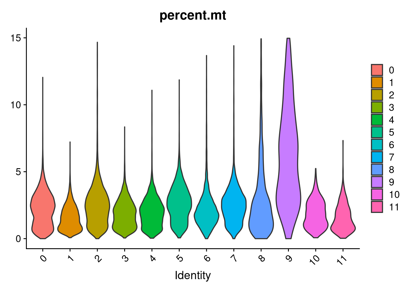
Clusters 9 and 6 were identified as non-microglial based on elevated mitochondrial content and non-microglial module scores. Their cell barcodes are saved here for removal in Part 2.
unwanted_cells <- WhichCells(merged_obj, idents = c("9", "6"))
length(unwanted_cells)
[1] 6020qs_save(unwanted_cells, file.path(objects_dir, "unwanted_cells_9_6.qs2"))sessionInfo()R version 4.5.1 (2025-06-13)
Platform: x86_64-pc-linux-gnu
Running under: Rocky Linux 8.7 (Green Obsidian)
Matrix products: default
BLAS/LAPACK: FlexiBLAS OPENBLAS; LAPACK version 3.12.0
locale:
[1] LC_CTYPE=en_GB.UTF-8 LC_NUMERIC=C
[3] LC_TIME=en_GB.UTF-8 LC_COLLATE=en_GB.UTF-8
[5] LC_MONETARY=en_GB.UTF-8 LC_MESSAGES=en_GB.UTF-8
[7] LC_PAPER=en_GB.UTF-8 LC_NAME=C
[9] LC_ADDRESS=C LC_TELEPHONE=C
[11] LC_MEASUREMENT=en_GB.UTF-8 LC_IDENTIFICATION=C
time zone: Europe/London
tzcode source: system (glibc)
attached base packages:
[1] stats4 stats graphics grDevices utils datasets methods
[8] base
other attached packages:
[1] ggrepel_0.9.6 scales_1.4.0
[3] presto_1.0.0 data.table_1.18.2.1
[5] Rcpp_1.1.1 qs2_0.1.6
[7] scDblFinder_1.24.10 SingleCellExperiment_1.32.0
[9] SummarizedExperiment_1.40.0 Biobase_2.70.0
[11] GenomicRanges_1.62.1 Seqinfo_1.0.0
[13] IRanges_2.44.0 S4Vectors_0.48.0
[15] BiocGenerics_0.56.0 generics_0.1.4
[17] MatrixGenerics_1.22.0 matrixStats_1.5.0
[19] SoupX_1.6.2 gridExtra_2.3
[21] future_1.70.0 readxl_1.4.5
[23] glue_1.8.0 lubridate_1.9.4
[25] forcats_1.0.1 stringr_1.6.0
[27] purrr_1.2.1 readr_2.1.6
[29] tidyr_1.3.2 tibble_3.3.1
[31] ggplot2_4.0.2 tidyverse_2.0.0
[33] Seurat_5.3.1.9001 SeuratObject_5.3.0.9003
[35] sp_2.2-1 Matrix_1.7-4
[37] dplyr_1.2.0
loaded via a namespace (and not attached):
[1] RcppAnnoy_0.0.23 splines_4.5.1
[3] later_1.4.6 BiocIO_1.20.0
[5] bitops_1.0-9 R.oo_1.27.1
[7] cellranger_1.1.0 polyclip_1.10-7
[9] XML_3.99-0.20 fastDummies_1.7.5
[11] lifecycle_1.0.5 edgeR_4.8.1
[13] globals_0.19.1 lattice_0.22-7
[15] MASS_7.3-65 magrittr_2.0.4
[17] limma_3.66.0 plotly_4.12.0
[19] rmarkdown_2.30 yaml_2.3.12
[21] metapod_1.18.0 httpuv_1.6.16
[23] otel_0.2.0 glmGamPoi_1.22.0
[25] sctransform_0.4.3 spam_2.11-3
[27] spatstat.sparse_3.1-0 reticulate_1.45.0
[29] cowplot_1.2.0 pbapply_1.7-4
[31] RColorBrewer_1.1-3 abind_1.4-8
[33] Rtsne_0.17 R.utils_2.13.0
[35] RCurl_1.98-1.17 irlba_2.3.7
[37] listenv_0.10.1 spatstat.utils_3.2-1
[39] goftest_1.2-3 RSpectra_0.16-2
[41] dqrng_0.4.1 spatstat.random_3.4-4
[43] fitdistrplus_1.2-6 parallelly_1.46.1
[45] DelayedMatrixStats_1.32.0 codetools_0.2-20
[47] DelayedArray_0.36.0 scuttle_1.20.0
[49] tidyselect_1.2.1 UCSC.utils_1.6.1
[51] farver_2.1.2 viridis_0.6.5
[53] ScaledMatrix_1.18.0 spatstat.explore_3.7-0
[55] GenomicAlignments_1.46.0 jsonlite_2.0.0
[57] BiocNeighbors_2.4.0 progressr_0.19.0
[59] scater_1.38.0 ggridges_0.5.7
[61] survival_3.8-3 systemfonts_1.3.1
[63] tools_4.5.1 ragg_1.5.0
[65] ica_1.0-3 SparseArray_1.10.8
[67] xfun_0.56 GenomeInfoDb_1.46.2
[69] withr_3.0.2 fastmap_1.2.0
[71] bluster_1.20.0 digest_0.6.39
[73] rsvd_1.0.5 timechange_0.3.0
[75] R6_2.6.1 mime_0.13
[77] textshaping_1.0.3 scattermore_1.2
[79] tensor_1.5.1 spatstat.data_3.1-9
[81] R.methodsS3_1.8.2 cigarillo_1.0.0
[83] rtracklayer_1.70.0 httr_1.4.8
[85] htmlwidgets_1.6.4 S4Arrays_1.10.1
[87] uwot_0.2.4 pkgconfig_2.0.3
[89] gtable_0.3.6 lmtest_0.9-40
[91] S7_0.2.1 XVector_0.50.0
[93] htmltools_0.5.9 dotCall64_1.2
[95] png_0.1-8 spatstat.univar_3.1-6
[97] scran_1.38.0 knitr_1.51
[99] tzdb_0.5.0 reshape2_1.4.5
[101] rjson_0.2.23 nlme_3.1-168
[103] curl_7.0.0 zoo_1.8-15
[105] KernSmooth_2.23-26 vipor_0.4.7
[107] parallel_4.5.1 miniUI_0.1.2
[109] ggrastr_1.0.2 restfulr_0.0.16
[111] pillar_1.11.1 grid_4.5.1
[113] vctrs_0.7.1 RANN_2.6.2
[115] promises_1.5.0 stringfish_0.17.0
[117] BiocSingular_1.26.1 beachmat_2.26.0
[119] xtable_1.8-4 cluster_2.1.8.1
[121] beeswarm_0.4.0 evaluate_1.0.5
[123] locfit_1.5-9.12 cli_3.6.5
[125] compiler_4.5.1 Rsamtools_2.26.0
[127] rlang_1.1.7 crayon_1.5.3
[129] future.apply_1.20.2 labeling_0.4.3
[131] ggbeeswarm_0.7.3 plyr_1.8.9
[133] stringi_1.8.7 viridisLite_0.4.3
[135] deldir_2.0-4 BiocParallel_1.44.0
[137] Biostrings_2.78.0 lazyeval_0.2.2
[139] spatstat.geom_3.7-0 RcppHNSW_0.6.0
[141] hms_1.1.4 patchwork_1.3.2
[143] sparseMatrixStats_1.22.0 statmod_1.5.1
[145] shiny_1.12.1 ROCR_1.0-12
[147] igraph_2.2.2 RcppParallel_5.1.11-1
[149] xgboost_3.2.0.1