GSEA (glmmTMB, trisomy)

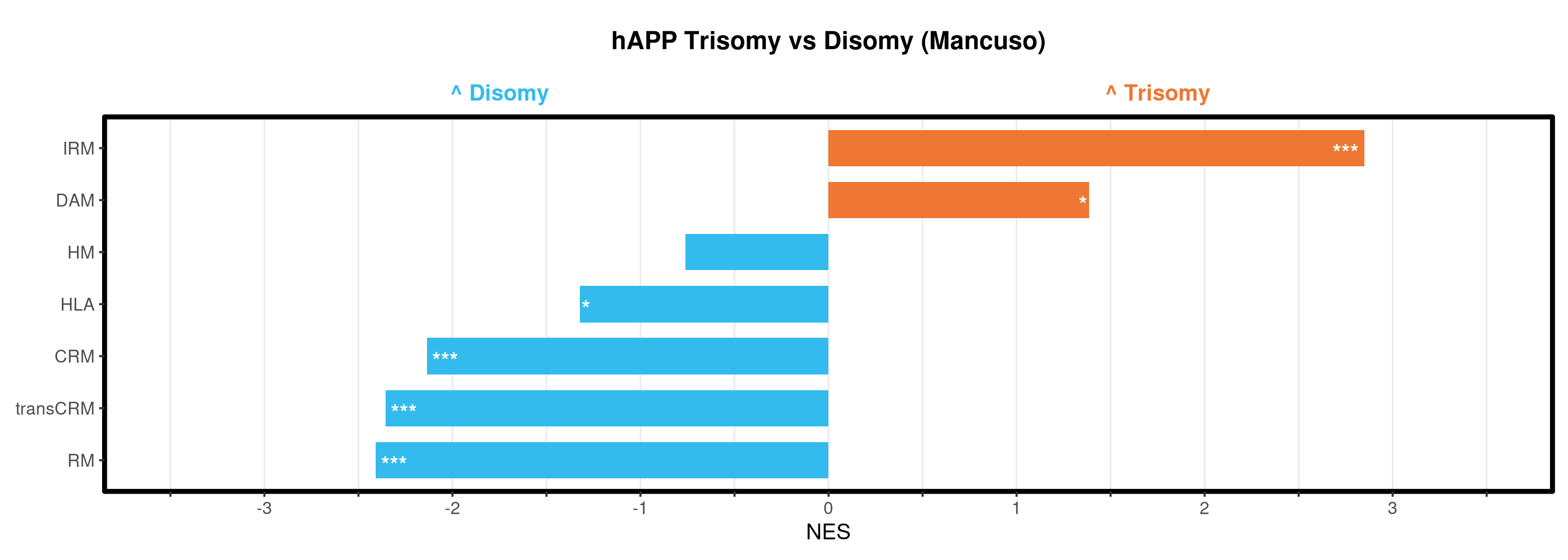
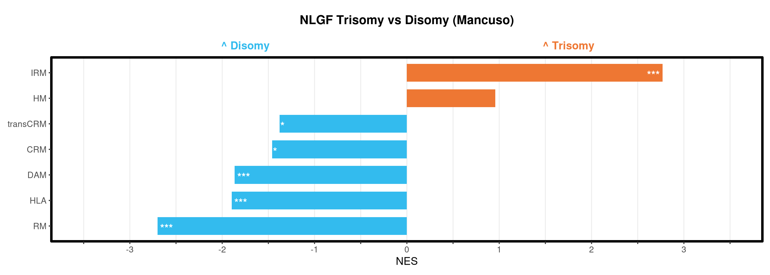
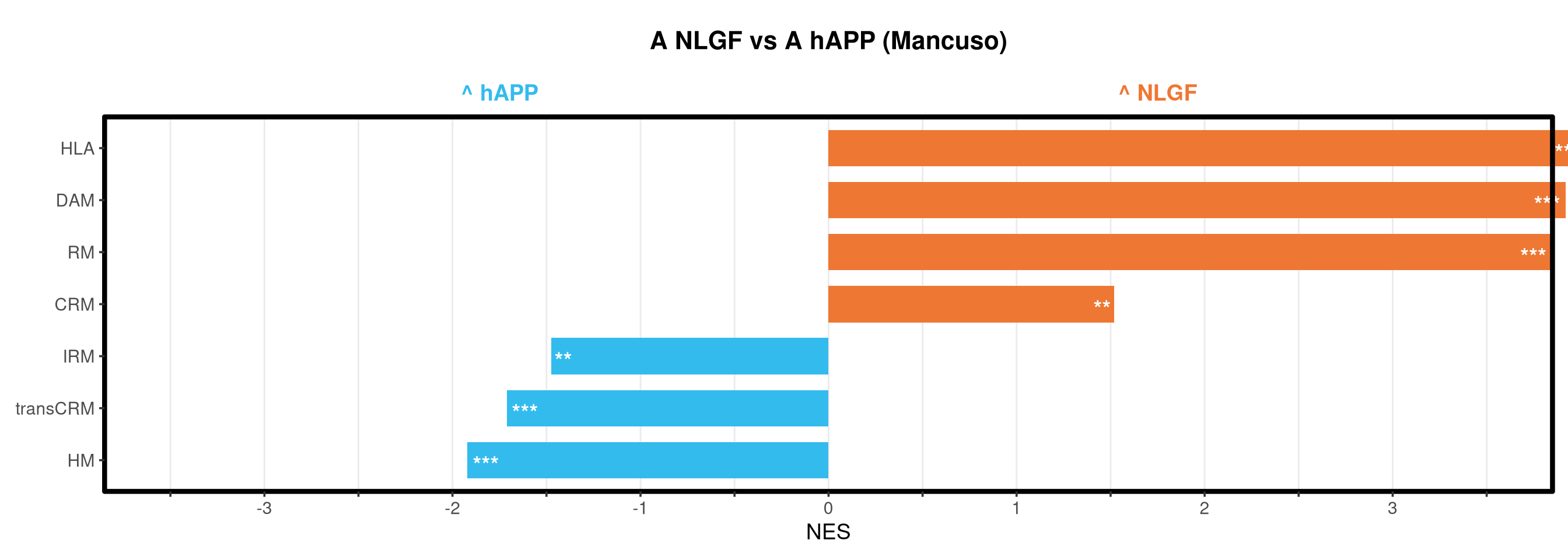
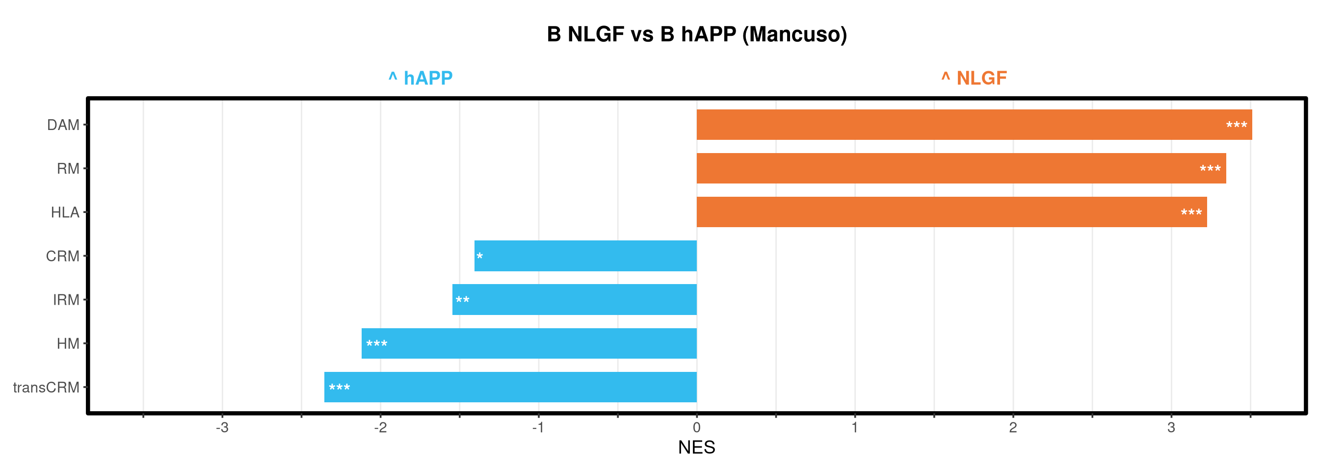
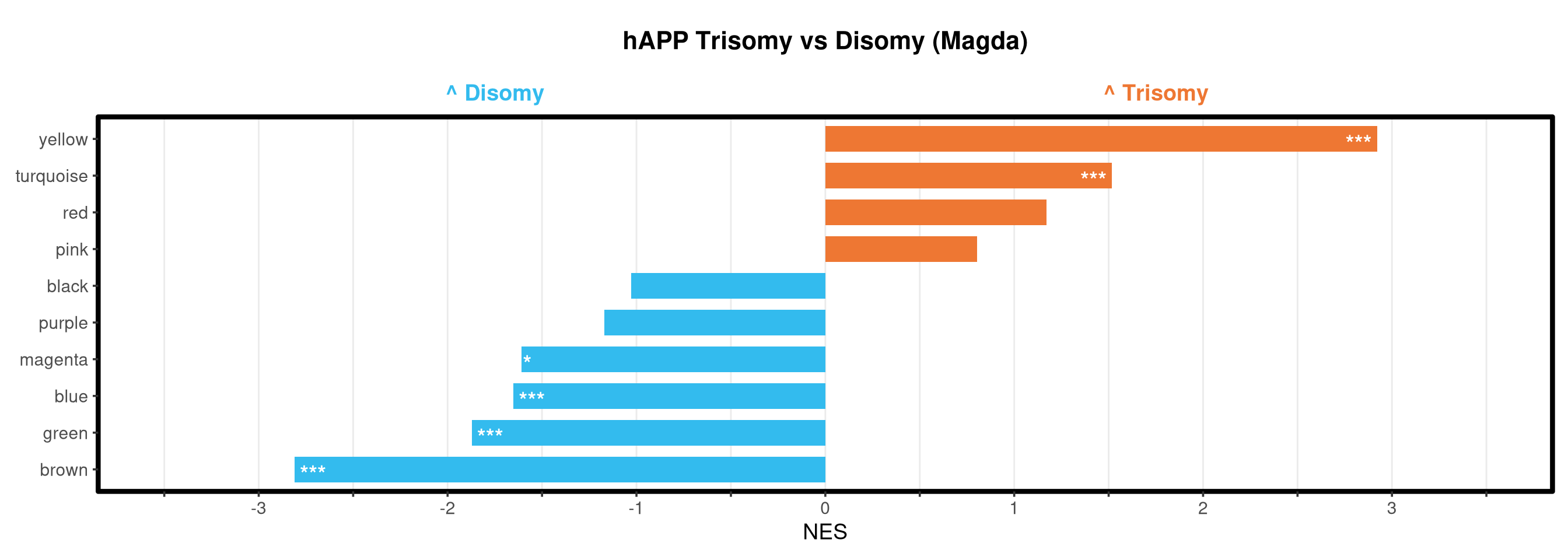
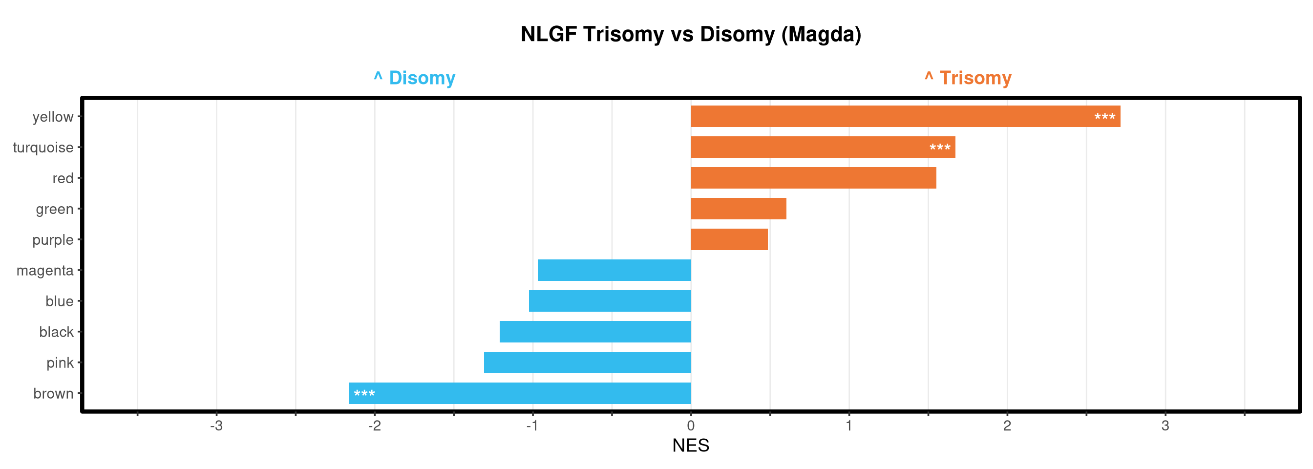
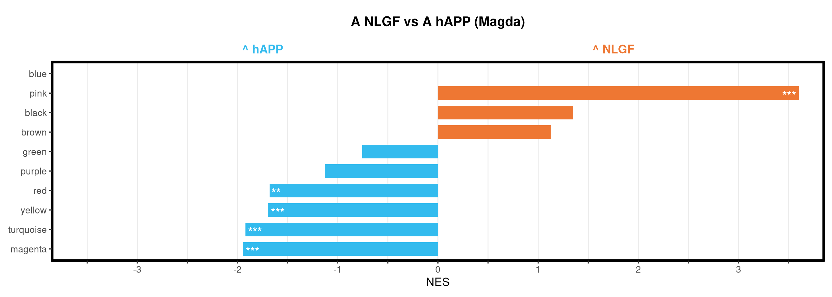
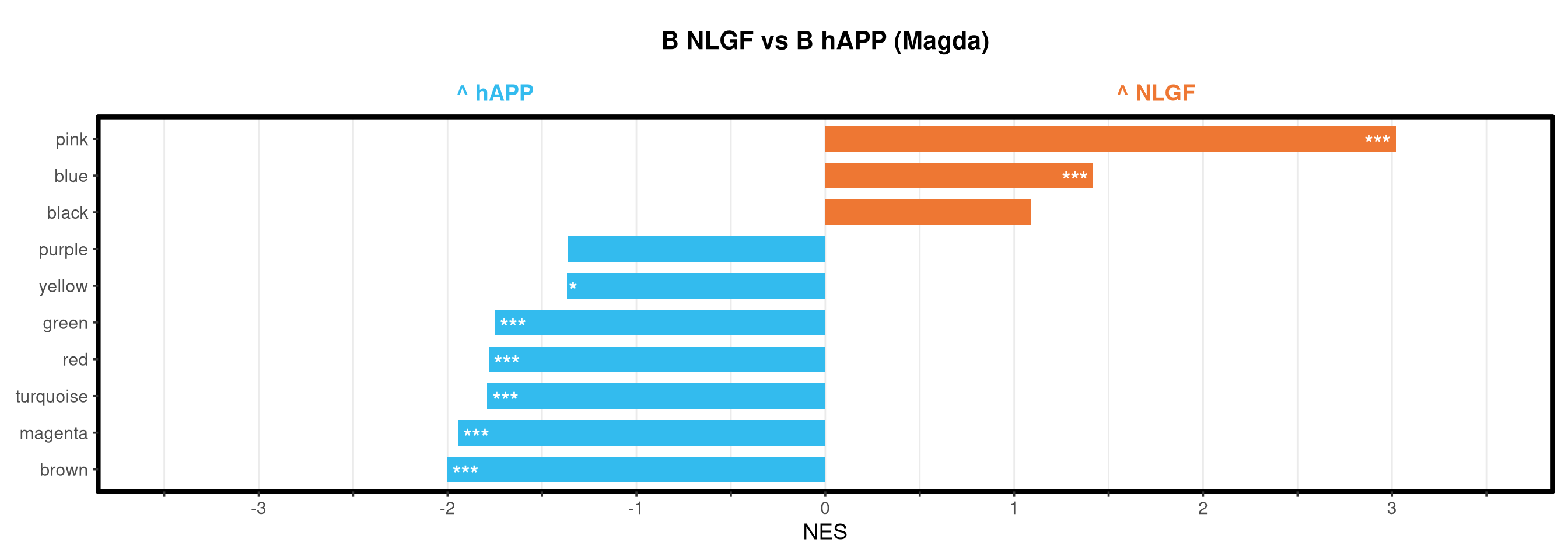
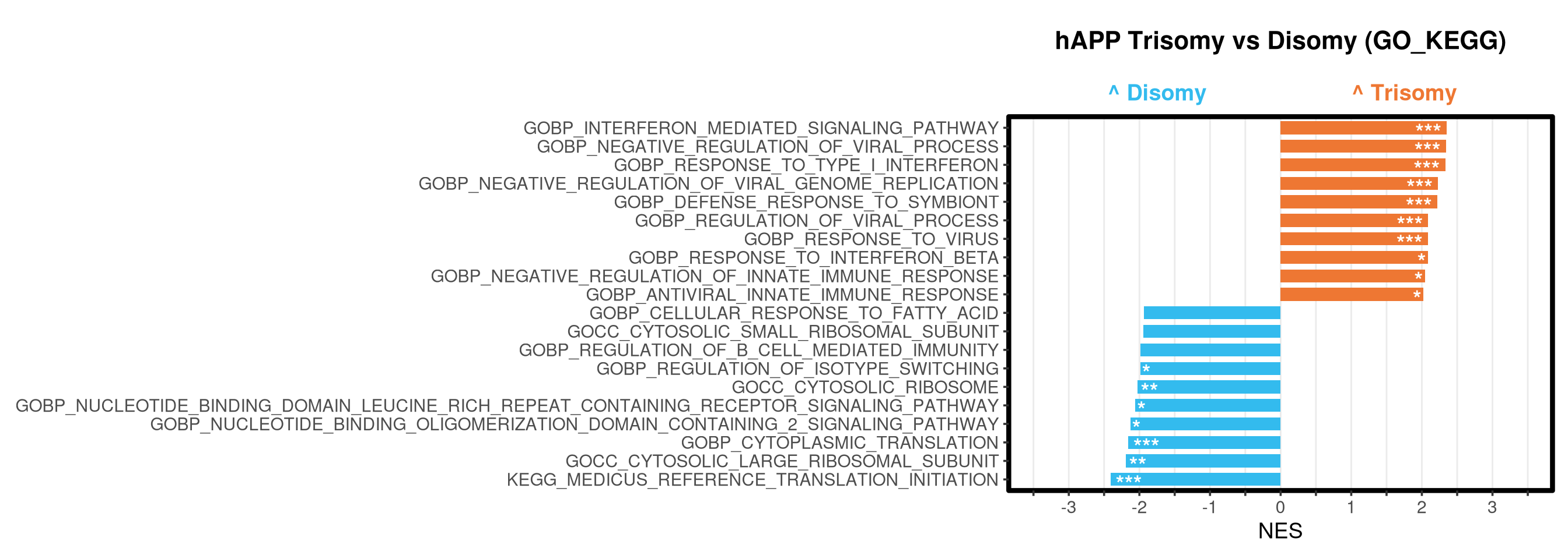
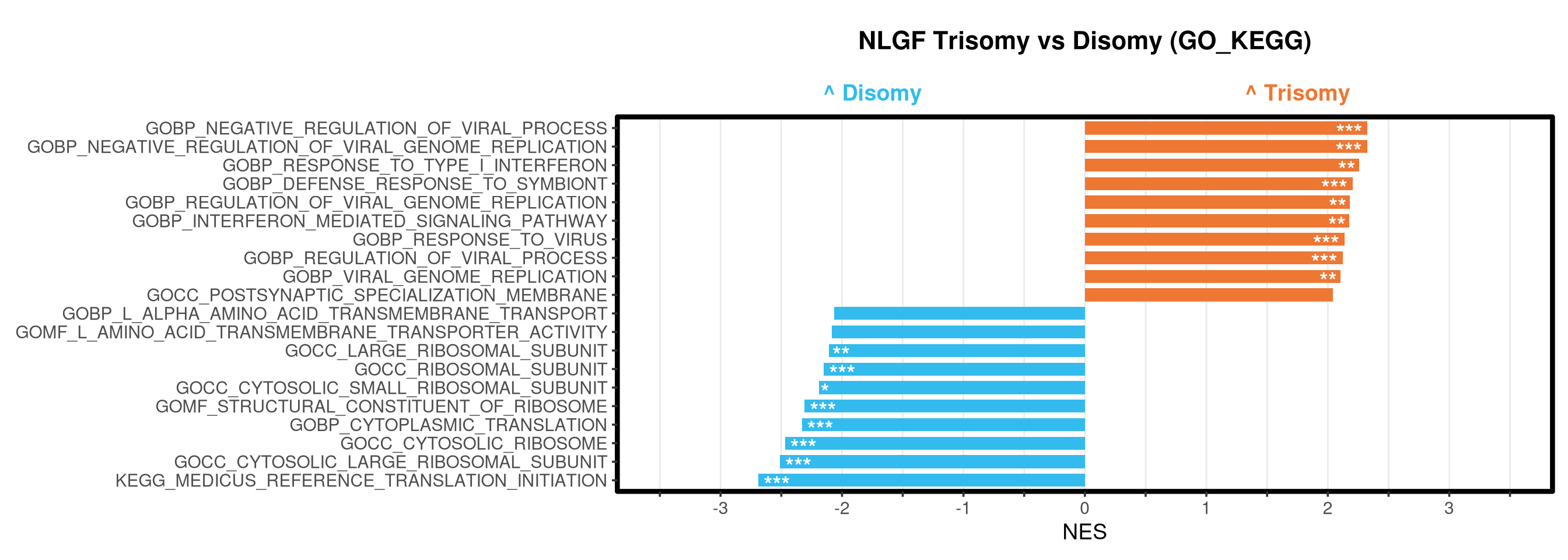
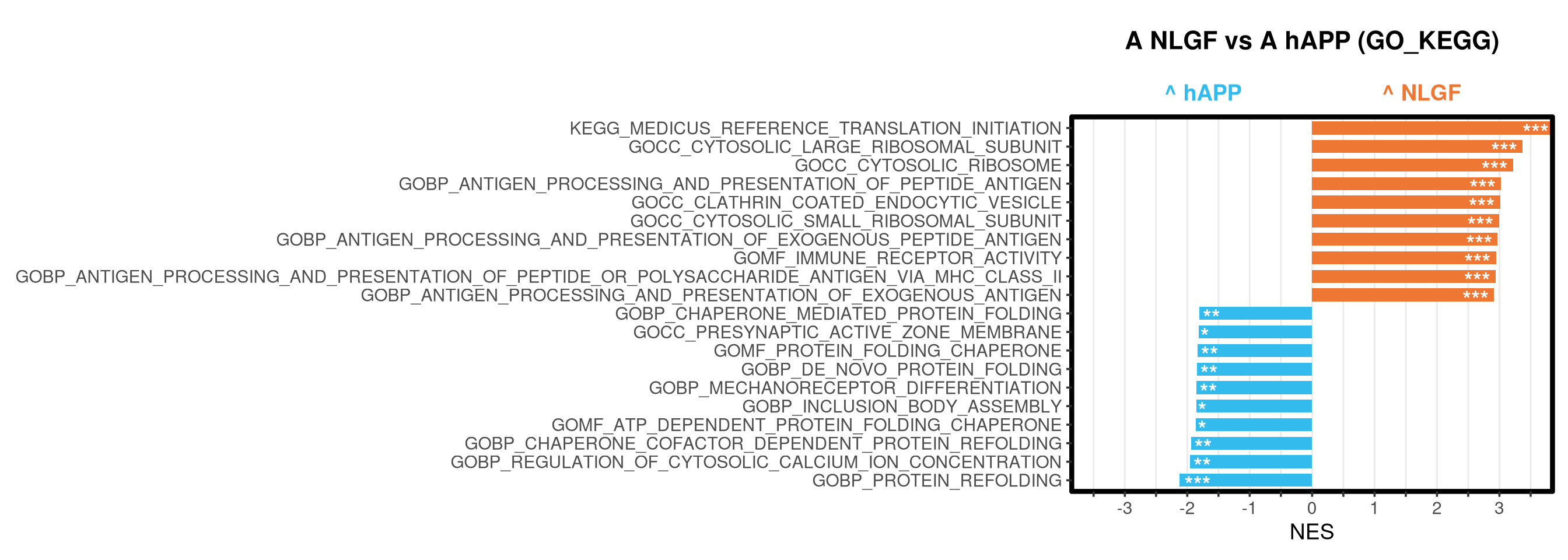
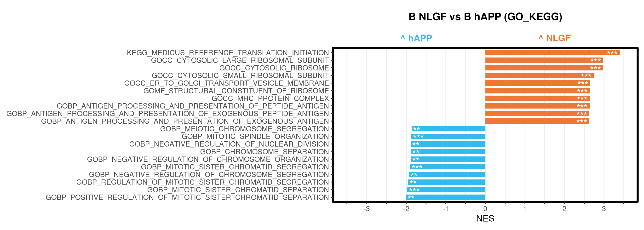
Runs gene set enrichment analysis (fgsea) on glmmTMB differential expression results across four contrasts: trisomy effect in hAPP and NLGF backgrounds, and background effect in trisomic and disomic cells. Gene sets include Mancuso 2024 signatures, custom module lists, and GO/KEGG pathways.

Inputs: output/run1/objects/glmmTMB_with_interactions_corrected.qs2; Mancuso geneset TXTs (../../Mancuso2024_genesets/); Magda modules Excel; GO/KEGG .gmt Outputs: CSV tables and barplot PDFs written to output/run1/glmmTMB/GSEA/

Load libraries

Code
library(SingleCellExperiment)
library(edgeR)
library(limma)
library(scuttle)
library(Seurat)
library(qs2)
library(ggrepel)
library(ggplot2)
library(stringr)
library(glue)
library(dplyr)
library(msigdbr)
library(fgsea)
library(viridis)
library(readxl)

Load directories

Code
run_num <- "run1"

out_dir <- file.path("output", run_num, "glmmTMB", "GSEA")
graphs_dir <- file.path(out_dir, "graphs")
objects_dir <- file.path(out_dir, "objects")

dir.create(graphs_dir, recursive = TRUE, showWarnings = FALSE)
dir.create(objects_dir, recursive = TRUE, showWarnings = FALSE)

Read in data

Code
required_input <- file.path("output", run_num, "objects", "glmmTMB_with_interactions_corrected.qs2")
if (!file.exists(required_input)) {
  message("Required input not found: ", required_input, "\nRun scripts/glmmTMB.qmd first.")
  knitr::knit_exit()
}
# 1. Load the finalized glmmTMB object
final_df <- qs_read(required_input)

Prepare rank vectors

Code
# 2. Define an upgraded ranking function tailored to your specific dataframe
create_glmm_rank <- function(df, target_background = NA, target_ploidy = NA, target_contrast) {
  
  # Filter based on which column has the context for the contrast
  if (!is.na(target_background)) {
    # e.g., Background == "hAPP" and contrast == "A - B"
    sub_df <- df %>% filter(Background == target_background & contrast == target_contrast)
  } else if (!is.na(target_ploidy)) {
    # e.g., Ploidy == "A" and contrast == "NLGF - hAPP"
    sub_df <- df %>% filter(Ploidy == target_ploidy & contrast == target_contrast)
  }
  
  if(nrow(sub_df) == 0) {
    stop(glue("No rows found. Check your target_background, target_ploidy, and target_contrast spelling!"))
  }
  
  # Calculate robust ranking metric: sign(log2FC) * -log10(p-value)
  # Adding 1e-300 prevents infinity errors if a p-value is exactly 0
  sub_df <- sub_df %>%
    mutate(rank_metric = log2FC)
  
  # Create the named vector required by fgsea
  ranks <- sub_df$rank_metric
  names(ranks) <- sub_df$Gene
  
  # Clean and sort
  ranks <- ranks[!is.na(ranks) & !is.na(names(ranks))]
  return(sort(ranks, decreasing = TRUE))
}

# 3. Create the Master List of Comparisons
comparisons_master <- list(
  "hAPP Trisomy vs Disomy"  = create_glmm_rank(final_df, target_background = "hAPP", target_contrast = "A - B"),
  "NLGF Trisomy vs Disomy"  = create_glmm_rank(final_df, target_background = "NLGF", target_contrast = "A - B"),
  "A NLGF vs A hAPP"        = create_glmm_rank(final_df, target_ploidy = "A",        target_contrast = "NLGF - hAPP"),
  "B NLGF vs B hAPP"        = create_glmm_rank(final_df, target_ploidy = "B",        target_contrast = "NLGF - hAPP")
)

GSEA function

Code
run_gsea_analysis <- function(ranks, 
                              comparison_name, 
                              geneset_name,    
                              pathways, 
                              base_objects_dir, 
                              base_graphs_dir,  
                              group_A_label = "Group A",
                              group_B_label = "Group B",
                              color_A = "#EE7733",
                              color_B = "#33BBEE") {
  
  message(glue("Running GSEA | Set: {geneset_name} | Comp: {comparison_name}"))
  
  # --- 1. Dynamic Directory Creation ---
  current_objects_dir <- file.path(base_objects_dir, "GSEA_Analysis", comparison_name)
  current_graphs_dir  <- file.path(base_graphs_dir, "GSEA_Analysis", comparison_name)
  
  dir.create(current_objects_dir, recursive = TRUE, showWarnings = FALSE)
  dir.create(current_graphs_dir, recursive = TRUE, showWarnings = FALSE)
  
  # --- 2. Run FGSEA ---
  set.seed(42)
  fgsea_res <- suppressMessages(fgsea(
    pathways = pathways,
    stats    = ranks,
    minSize  = 15,
    maxSize  = 3000,
    nproc    = 1,
    BPPARAM  = BiocParallel::SerialParam(progressbar = FALSE)
  ))
  
  if (nrow(fgsea_res) == 0) {
    warning(glue("No significant pathways for {geneset_name} in {comparison_name}"))
    return(NULL)
  }
  
  # --- 3. Save CSV ---
  fgsea_res_tidy <- fgsea_res %>%
    as_tibble() %>%
    mutate(leadingEdge = sapply(leadingEdge, paste, collapse = ",")) %>%
    # Clean Pathway Names
    mutate(pathway = gsub("_geneset", "", pathway)) %>% 
    arrange(padj)
  
  csv_name <- glue("Table_{geneset_name}.csv")
  write.csv(fgsea_res_tidy, file.path(current_objects_dir, csv_name), row.names = FALSE)
  
  # --- 4. Plotting ---
  top_gsea <- fgsea_res_tidy %>%
    arrange(desc(NES)) %>%
    slice_head(n = 10) %>%
    bind_rows(fgsea_res_tidy %>% arrange(NES) %>% slice_head(n = 10)) %>%
    distinct(pathway, .keep_all = TRUE) %>%
    mutate(
      sig_label = case_when(
        padj < 0.001 ~ "***",
        padj < 0.01  ~ "**",
        padj < 0.05  ~ "*",
        TRUE         ~ ""
      ),
      fill_group = ifelse(NES > 0, group_A_label, group_B_label),
      pathway = factor(pathway, levels = unique(pathway[order(NES)]))
    )
  
  if (nrow(top_gsea) == 0) return(fgsea_res_tidy)
  
  # Hard axis limit
  axis_zoom <- 3.5 
  
  plot_title <- glue("{sub('_.*', '', comparison_name)} ({geneset_name})")
  
  p <- ggplot(top_gsea, aes(x = NES, y = pathway, fill = fill_group)) +
    
    # 1. Add faint vertical grid lines BEHIND bars (using geom_vline or theme)
    # The cleanest way is usually via theme, but here is the setup:
    geom_col(width = 0.7) +
    
    geom_text(aes(label = sig_label, hjust = ifelse(NES > 0, 1.2, -0.2)), 
              color = "white", size = 5, vjust = 0.75, fontface = "bold") +
    
    scale_fill_manual(values = setNames(c(color_A, color_B), c(group_A_label, group_B_label))) +
    
    # --- AXIS CONFIGURATION ---
    scale_x_continuous(
      # Create breaks at every 0.5 interval
      breaks = seq(-axis_zoom, axis_zoom, 0.5),
      # Custom label function: If x is an integer, show x. Else show empty string.
      labels = function(x) ifelse(x %% 1 == 0, x, "")
    ) +
    scale_y_discrete(labels = function(x) str_wrap(x, width = 40)) +

    labs(x = "NES", y = NULL, title = plot_title) +
    theme_bw(base_size = 14) +
    
    theme(
      # Turn ON vertical grid lines (major.x), make them faint grey
      panel.grid.major.x = element_line(color = "grey92", linewidth = 0.5),
      # Turn OFF horizontal grid lines (major.y) and minor grids
      panel.grid.major.y = element_blank(),
      panel.grid.minor   = element_blank(),
      
      panel.border = element_rect(colour = "black", fill = NA, linewidth = 1.5),
      legend.position = "none",
      
      plot.title = element_text(hjust = 0.5, face = "bold", size = 16, margin = margin(b = 40)),
      
      # Adjust top margin (t) slightly to ensure title isn't cut off at the very top of PDF
      plot.margin = margin(t = 20, r = 10, b = 10, l = 10, unit = "pt")
    ) +
    
    # Annotations
    annotate("text", x = -axis_zoom/2, y = Inf, 
             label = glue("^ {group_B_label}"), color = color_B, size = 5, fontface = "bold", vjust = -1.0) +
    annotate("text", x = axis_zoom/2, y = Inf, 
             label = glue("^ {group_A_label}"), color = color_A, size = 5, fontface = "bold", vjust = -1.0) +
    
    coord_cartesian(xlim = c(-axis_zoom, axis_zoom), clip = "off")
  
  # --- 5. Save Plot ---
  plot_name <- glue("Barplot_{geneset_name}.pdf")
  
  # Calculate Height: Base 2 inches + 0.3 inches per bar
  dynamic_height <- 2 + (nrow(top_gsea) * 0.3)
  
  # NEW: Calculate Width based on the longest label text
  # 1. Find the longest pathway name (number of characters)
  max_len <- max(nchar(as.character(top_gsea$pathway)))
  
  # 2. Set width: 5 inches for the plot bars + roughly 0.12 inches per character of text
  #    Examples: 
  #    - Short names (10 chars) -> 5 + 1.2 = ~6.2 inches wide
  #    - Long GO terms (60 chars) -> 5 + 7.2 = ~12.2 inches wide
  dynamic_width <- 5 + (max_len * 0.12)
  
  ggsave(filename = file.path(current_graphs_dir, plot_name),
         plot = p,
         width = dynamic_width,
         height = dynamic_height,
         limitsize = FALSE) # Allows creating very large PDFs if needed

  print(p)

  return(fgsea_res_tidy)
}

Config and gene sets

Code
# --- A. General Settings ---
GLOBAL_CONFIG <- list(
  output_dir = file.path(out_dir, "GSEA_Results_Master"), 
  group_A    = "Group A",
  group_B    = "Group B",
  col_A      = "#EE7733",
  col_B      = "#33BBEE"
)

# --- B. Load Gene Sets ---

# 1. Mancuso (TXT files)
mancuso_dir <- "../../Mancuso2024_genesets"
mancuso_files <- list.files(path = mancuso_dir, pattern = "\\.txt$")
mancuso_list <- lapply(mancuso_files, function(x) {
  scan(file.path(mancuso_dir, x), what = "character", quiet = TRUE)
})
names(mancuso_list) <- gsub(".txt$", "", mancuso_files)

# 2. Magda (Excel)
module_data <- read_excel("/camp/home/zanettc/home/shared/zanettc/external_data/magda_modules.xlsx")
magda_list <- lapply(module_data, function(x) unique(na.omit(as.character(x))))
magda_list <- magda_list[sapply(magda_list, length) > 0] 

#3. GO / KEGG
go_pathways <- gmtPathways("../../GO_human_all_genesets.gmt")
kegg_df <- msigdbr(species = "Homo sapiens", collection = "C2", subcollection = "CP:KEGG_MEDICUS")
kegg_list <- split(x = kegg_df$gene_symbol, f = kegg_df$gs_name)
go_kegg_list <- c(go_pathways, kegg_list)


# 3. Master List
gene_sets_master <- list(
  "Mancuso" = mancuso_list,
  "Magda"   = magda_list,
  "GO_KEGG" = go_kegg_list
)

Execution loop

Code
purrr::walk2(names(gene_sets_master), gene_sets_master, function(gset_name, gset_pathways) {
  purrr::walk2(comparisons_master, names(comparisons_master), function(ranks, comp_name) {
    
    # 1. Dynamically determine group labels based on the current comparison name
    # Ensure Group A corresponds to the positive side of your contrast (e.g., "A" or "NLGF")
    # and Group B corresponds to the negative side (e.g., "B" or "hAPP")
    if (str_detect(comp_name, "Trisomy vs Disomy")) {
      label_A <- "Trisomy"
      label_B <- "Disomy"
    } else if (str_detect(comp_name, "NLGF vs.*hAPP")) {
      label_A <- "NLGF"
      label_B <- "hAPP"
    } else {
      # Fallback just in case a new comparison is added later
      label_A <- "Group A"
      label_B <- "Group B"
    }

    # 2. Pass the dynamic labels into the GSEA function
    run_gsea_analysis(
      ranks            = ranks,
      comparison_name  = comp_name,
      geneset_name     = gset_name,      
      pathways         = gset_pathways, 
      base_objects_dir = objects_dir,   
      base_graphs_dir  = graphs_dir,    
      group_A_label    = label_A,
      group_B_label    = label_B,
      color_A          = GLOBAL_CONFIG$col_A,
      color_B          = GLOBAL_CONFIG$col_B
    )
    
    gc() # Memory cleanup
  })
})

Single pathway enrichment plot

Code
term_to_plot <- "KEGG_MEDICUS_REFERENCE_TRANSLATION_INITIATION"

# 1. Flatten your master gene set list so we can find the term easily
#    (unname prevents "GO_KEGG.TermName" prefixes)
all_pathways_flat <- do.call(c, unname(gene_sets_master))

# 2. Check if the term exists before looping
if (!term_to_plot %in% names(all_pathways_flat)) {
  stop(glue("Could not find pathway '{term_to_plot}' in gene_sets_master."))
}

pathway_genes <- all_pathways_flat[[term_to_plot]]

# 3. Create a specific output folder
specific_graphs_dir <- file.path(graphs_dir, "Specific_Pathway_Plots")
dir.create(specific_graphs_dir, showWarnings = FALSE, recursive = TRUE)

# 4. Loop and Plot
purrr::walk2(comparisons_master, names(comparisons_master), function(ranks, comp_name) {
  
  message(glue("Plotting {term_to_plot} for {comp_name}..."))
  
  # Generate the GSEA enrichment plot
  gsea_plot <- plotEnrichment(pathway_genes, ranks) +
    labs(
      title = term_to_plot,
      subtitle = glue("Comparison: {comp_name}"),
      x = "Rank",
      y = "Enrichment Score"
    ) +
    theme_bw(base_size = 14) +
    theme(
      plot.title = element_text(face = "bold", hjust = 0.5),
      plot.subtitle = element_text(hjust = 0.5, color = "grey40"),
      panel.grid = element_blank()
    )
  
  # Save
  ggsave(
    filename = file.path(specific_graphs_dir, glue("{term_to_plot}_{comp_name}.pdf")),
    plot = gsea_plot,
    width = 8, 
    height = 5
  )
})

Combined GSEA plots

Define function

Code
plot_combined_gsea <- function(pathway_name, rank_list, pathways_obj, graphs_dir) {
  
  # --- A. Sanitize Filename ---
  safe_pathway_name <- gsub("[[:punct:]]", "_", pathway_name)
  
  # --- B. Check if pathway exists ---
  if (!pathway_name %in% names(pathways_obj)) {
    warning(glue("Pathway '{pathway_name}' not found in the provided pathway object."))
    return(NULL)
  }
  
  gene_set <- pathways_obj[[pathway_name]]
  plot_data_list <- list()
  
  # --- C. Loop through comparisons ---
  for (comp_name in names(rank_list)) {
    
    ranks <- rank_list[[comp_name]]
    
    # Generate the standard fgsea plot object
    # Note: We suppress messages to avoid "calibrating stats" spam
    g <- suppressMessages(plotEnrichment(gene_set, ranks))
    
    # Extract the data frame (columns are typically 'rank' and 'ES')
    df <- g$data
    df$Comparison <- comp_name 
    
    plot_data_list[[comp_name]] <- df
  }
  
  # --- D. Combine data ---
  combined_df <- bind_rows(plot_data_list)
  
  # --- E. Plot ---
  p <- ggplot(combined_df, aes(x = rank, y = ES, color = Comparison)) +
    geom_line(linewidth = 1.2, alpha = 0.8) +
    
    # Add zero line for reference
    geom_hline(yintercept = 0, linetype = "dashed", color = "grey60") +
    
    labs(
      title = pathway_name,
      x = "Gene Rank",
      y = "Enrichment Score"
    ) +
    
    # Use distinct colors for the different comparisons (hAPP vs NLGF)
    scale_color_brewer(palette = "Set1") +
    
    theme_bw(base_size = 14) +
    theme(
      legend.position = "bottom",
      plot.title = element_text(size = 14, face = "bold", hjust = 0.5),
      panel.grid.minor = element_blank()
    )
  
  # --- F. Save ---
  # Create a subfolder for these combined plots
  combined_out_dir <- file.path(graphs_dir, "Combined_GSEA_Plots")
  dir.create(combined_out_dir, showWarnings = FALSE, recursive = TRUE)
  
  file_name <- file.path(combined_out_dir, glue("{safe_pathway_name}_Combined.pdf"))
  
  ggsave(filename = file_name, plot = p, width = 8, height = 6)
  
  return(p)
}

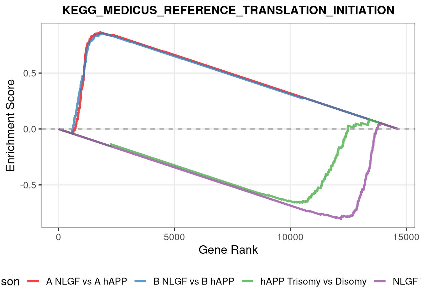
Combined enrichment — specific term

Code
term_to_plot <- "KEGG_MEDICUS_REFERENCE_TRANSLATION_INITIATION"

# 1. Flatten the master list so we can search all pathways at once
all_pathways_flat <- do.call(c, unname(gene_sets_master))

combined_plot <- plot_combined_gsea(
  pathway_name = term_to_plot,
  rank_list    = comparisons_master,  # Uses your hAPP and NLGF ranks
  pathways_obj = all_pathways_flat,   # Uses the flattened list
  graphs_dir   = graphs_dir
)

print(combined_plot)