10. Aβ tryptic peptide correlation

Identify proteins whose MSstats-summarised abundance tracks the Aβ tryptic peptide (LVFFAEDVGSNK) signal across samples.

Primary analysis is restricted to plaque_near — asks “within plaque regions, what co-varies with Aβ load?”. A secondary plaque_near + plaque_far analysis serves as a sensitivity check with wider dynamic range.

Libraries

Code

suppressPackageStartupMessages({
  library(data.table)
  library(qs2)
  library(dplyr)
  library(tidyr)
  library(tibble)
  library(ggplot2)
  library(ggrepel)
  library(purrr)
})

Directories

Code

base_dir <- "/nemo/lab/destrooperb/home/shared/zanettc/millie_proteomics"
run_num <- "run5"

results_dir <- file.path(base_dir, "results", run_num)
objects_dir <- file.path(base_dir, "data", "processed", run_num)
graphs_dir <- file.path(results_dir, "ab_correlation")

dir.create(graphs_dir, recursive = TRUE, showWarnings = FALSE)

Load protein-level data and build wide matrix

Code

processed_data <- qs_read(file.path(objects_dir, "processed_msstats_data.qs2"))

protein_dict <- fread(file.path(base_dir, "data/processed/run1/clean_spec_raw.csv")) %>%
  dplyr::select(Protein = PG.ProteinGroups, Gene = PG.Genes) %>%
  distinct()

wide_df <- processed_data$ProteinLevelData %>%
  left_join(protein_dict, by = "Protein") %>%
  mutate(Gene = ifelse(is.na(Gene) | Gene == "", Protein, Gene)) %>%
  group_by(originalRUN, Gene) %>%
  summarize(Abundance = mean(LogIntensities, na.rm = TRUE), .groups = "drop") %>%
  pivot_wider(names_from = Gene, values_from = Abundance) %>%
  column_to_rownames("originalRUN")

cat("Wide matrix: ", nrow(wide_df), "runs x ", ncol(wide_df), "genes\n")

Wide matrix:  82 runs x  5563 genes

Build Aβ peptide target vector

Sum fragment-level F.PeakArea across all precursors of LVFFAEDVGSNK per run, then log2-transform. Runs not covered by the clean msstats data are dropped.

Code

target_peptide <- "LVFFAEDVGSNK"

msstats_clean <- qs_read(file.path(base_dir, "data/processed/run1/clean_msstats_input.qs2"))

ab_target <- as.data.table(msstats_clean)[
    PEP.StrippedSequence == target_peptide,
    .(ab_intensity = sum(F.PeakArea, na.rm = TRUE)),
    by = R.FileName
  ] %>%
  as_tibble() %>%
  mutate(Ab_log2 = log2(ab_intensity + 1)) %>%
  dplyr::rename(Run = R.FileName) %>%
  dplyr::select(Run, Ab_log2)

rm(msstats_clean); invisible(gc())

cat("Aβ target vector: ", nrow(ab_target), "runs\n")

Aβ target vector:  159 runs

Code

summary(ab_target$Ab_log2)

   Min. 1st Qu.  Median    Mean 3rd Qu.    Max. 
  2.397   6.329   7.398   7.641   8.601  12.531

Metadata and sample sets

Code

final_clean_meta <- read.csv(file.path(base_dir, "data/processed/run1/msstats_annotation.csv"))

near_runs    <- final_clean_meta$Run[final_clean_meta$Condition == "plaque_near"]
nearfar_runs <- final_clean_meta$Run[final_clean_meta$Condition %in% c("plaque_near", "plaque_far")]

cat("plaque_near runs:", length(near_runs), "\n")

plaque_near runs: 24

Code

cat("plaque_near + plaque_far runs:", length(nearfar_runs), "\n")

plaque_near + plaque_far runs: 53

Code

# Intersect with the runs that actually have an Aβ measurement
cat("plaque_near with Aβ signal:",      sum(near_runs    %in% ab_target$Run), "\n")

plaque_near with Aβ signal: 24

Code

cat("near+far with Aβ signal:",          sum(nearfar_runs %in% ab_target$Run), "\n")

near+far with Aβ signal: 53

Correlation function (Pearson + Spearman + FDR)

Code

correlate_to_ab <- function(sample_runs, wide_df, ab_target, min_n = 4) {

  runs_keep <- intersect(intersect(sample_runs, rownames(wide_df)), ab_target$Run)
  if (length(runs_keep) < min_n) {
    stop("Fewer than ", min_n, " samples available for correlation.")
  }

  data_sub <- wide_df[runs_keep, , drop = FALSE]
  ab_vec   <- ab_target$Ab_log2[match(runs_keep, ab_target$Run)]

  genes <- colnames(data_sub)

  results <- map_dfr(genes, function(g) {
    x <- data_sub[[g]]
    y <- ab_vec
    keep <- !is.na(x) & !is.na(y)
    n <- sum(keep)
    if (n < min_n) return(NULL)

    # Guard against zero-variance vectors (Spearman/Pearson throw warnings)
    if (sd(x[keep]) == 0 || sd(y[keep]) == 0) return(NULL)

    p_test <- suppressWarnings(cor.test(x[keep], y[keep], method = "pearson"))
    s_test <- suppressWarnings(cor.test(x[keep], y[keep], method = "spearman",
                                        exact = FALSE))

    tibble(
      Gene         = g,
      n_pairs      = n,
      Pearson_R    = unname(p_test$estimate),
      Pearson_p    = p_test$p.value,
      Spearman_rho = unname(s_test$estimate),
      Spearman_p   = s_test$p.value
    )
  })

  results %>%
    mutate(
      Pearson_FDR  = p.adjust(Pearson_p,  method = "BH"),
      Spearman_FDR = p.adjust(Spearman_p, method = "BH")
    ) %>%
    arrange(desc(Pearson_R))
}

Primary analysis: plaque_near

Code

ab_cors_near <- correlate_to_ab(near_runs, wide_df, ab_target)

cat("Primary analysis: ", nrow(ab_cors_near), "genes correlated, n_pairs =",
    unique(ab_cors_near$n_pairs), "\n\n")

Primary analysis:  5563 genes correlated, n_pairs = 12 24 23 22 19 21 9 20 14 18 16 6 17 15 13 10 11 8 5 7

Code

head(ab_cors_near, 20)

Code

tail(ab_cors_near, 20)

Code

write.csv(ab_cors_near,
          file.path(objects_dir, "ab_correlation_near.csv"),
          row.names = FALSE)

Secondary (sensitivity check): plaque_near + plaque_far

Code

ab_cors_nearfar <- correlate_to_ab(nearfar_runs, wide_df, ab_target)

cat("Sensitivity analysis: ", nrow(ab_cors_nearfar), "genes correlated, n_pairs =",
    unique(ab_cors_nearfar$n_pairs), "\n\n")

Sensitivity analysis:  5563 genes correlated, n_pairs = 52 53 50 47 49 27 51 48 46 42 41 22 30 23 45 17 34 16 38 18 44 28 36 43 31 21 25 33 24 37 40 19 35 26 20 32 39 29 15

Code

head(ab_cors_nearfar, 20)

Code

tail(ab_cors_nearfar, 20)

Code

write.csv(ab_cors_nearfar,
          file.path(objects_dir, "ab_correlation_near_far.csv"),
          row.names = FALSE)

Concordance between the two analyses

Top hits that survive both are the most defensible candidates.

Code

concord <- ab_cors_near %>%
  dplyr::select(Gene,
                R_near = Pearson_R,
                p_near = Pearson_p,
                FDR_near = Pearson_FDR) %>%
  inner_join(
    ab_cors_nearfar %>%
      dplyr::select(Gene,
                    R_nearfar = Pearson_R,
                    p_nearfar = Pearson_p,
                    FDR_nearfar = Pearson_FDR),
    by = "Gene"
  ) %>%
  arrange(desc(R_near))

ggplot(concord, aes(R_near, R_nearfar)) +
  geom_hline(yintercept = 0, colour = "grey70") +
  geom_vline(xintercept = 0, colour = "grey70") +
  geom_point(alpha = 0.4, size = 1) +
  geom_abline(slope = 1, intercept = 0, linetype = "dashed", colour = "red") +
  geom_text_repel(
    data = concord %>% filter(abs(R_near) > 0.8 & abs(R_nearfar) > 0.6),
    aes(label = Gene), size = 3, max.overlaps = 30
  ) +
  labs(
    title = "Pearson R concordance: plaque_near vs plaque_near+plaque_far",
    x = "Pearson R (plaque_near only)",
    y = "Pearson R (plaque_near + plaque_far)"
  ) +
  theme_minimal()

Warning: ggrepel: 22 unlabeled data points (too many overlaps). Consider
increasing max.overlaps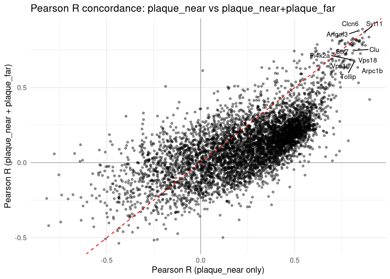

Code

ggsave(file.path(graphs_dir, "concordance_R_near_vs_nearfar.pdf"),
       width = 8, height = 7)

Warning: ggrepel: 12 unlabeled data points (too many overlaps). Consider
increasing max.overlaps

Volcano: Pearson R vs -log10(p) — primary analysis

Code

volcano_df <- ab_cors_near %>%
  mutate(neg_log10_p = -log10(Pearson_p),
         sig = case_when(
           Pearson_FDR < 0.05 & Pearson_R > 0 ~ "Pos (FDR<0.05)",
           Pearson_FDR < 0.05 & Pearson_R < 0 ~ "Neg (FDR<0.05)",
           Pearson_p  < 0.05 & Pearson_R > 0  ~ "Pos (p<0.05)",
           Pearson_p  < 0.05 & Pearson_R < 0  ~ "Neg (p<0.05)",
           TRUE                                ~ "n.s."
         ))

top_labels <- volcano_df %>%
  filter(Pearson_p < 0.05) %>%
  slice_max(order_by = abs(Pearson_R), n = 30)

ggplot(volcano_df, aes(Pearson_R, neg_log10_p, colour = sig)) +
  geom_point(alpha = 0.5, size = 1) +
  geom_vline(xintercept = 0, colour = "grey70") +
  geom_hline(yintercept = -log10(0.05), linetype = "dashed", colour = "grey50") +
  geom_text_repel(
    data = top_labels,
    aes(label = Gene),
    size = 3, max.overlaps = 35,
    box.padding = 0.4, segment.alpha = 0.5
  ) +
  scale_colour_manual(values = c(
    "Pos (FDR<0.05)" = "#d95f02",
    "Neg (FDR<0.05)" = "#1b9e77",
    "Pos (p<0.05)"   = "#fdb462",
    "Neg (p<0.05)"   = "#8dd3c7",
    "n.s."           = "grey70"
  )) +
  labs(
    title = paste0("Correlation of protein abundance with Aβ peptide (",
                   target_peptide, ")"),
    subtitle = "plaque_near samples",
    x = "Pearson R",
    y = "-log10(p)"
  ) +
  theme_minimal() +
  theme(legend.title = element_blank())

Code

ggsave(file.path(graphs_dir, "volcano_ab_correlation_near.pdf"),
       width = 10, height = 7)

Warning in grid.Call.graphics(C_text, as.graphicsAnnot(x$label), x$x, x$y, :
conversion failure on 'Correlation of protein abundance with Aβ peptide
(LVFFAEDVGSNK)' in 'mbcsToSbcs': for β (U+03B2)

Sanity-check scatter plots for known markers

Code

marker_genes <- c("Gfap", "App", "Apoe", "Clu", "C1qa", "C1qb", "C1qc",
                  "Trem2", "Cd44", "Vim", "S100b")
marker_genes <- intersect(marker_genes, colnames(wide_df))

scatter_runs <- intersect(nearfar_runs, ab_target$Run)
scatter_runs <- intersect(scatter_runs, rownames(wide_df))

scatter_df <- tibble(Run = scatter_runs) %>%
  mutate(Ab_log2 = ab_target$Ab_log2[match(Run, ab_target$Run)]) %>%
  left_join(final_clean_meta %>% dplyr::select(Run, Condition), by = "Run")

for (g in marker_genes) {
  scatter_df[[g]] <- wide_df[scatter_df$Run, g]
}

scatter_long <- scatter_df %>%
  pivot_longer(cols = all_of(marker_genes),
               names_to = "Gene",
               values_to = "LogIntensity")

# Compute per-gene R within plaque_near only, for the panel annotations
anno_df <- scatter_long %>%
  filter(Condition == "plaque_near") %>%
  group_by(Gene) %>%
  summarise(
    R = cor(Ab_log2, LogIntensity, use = "pairwise.complete.obs"),
    .groups = "drop"
  ) %>%
  mutate(label = sprintf("R[near] = %.2f", R))

ggplot(scatter_long, aes(Ab_log2, LogIntensity, colour = Condition)) +
  geom_point(size = 2, alpha = 0.8) +
  geom_smooth(data = scatter_long %>% filter(Condition == "plaque_near"),
              aes(group = 1), method = "lm", se = FALSE,
              colour = "black", linewidth = 0.6) +
  geom_text(data = anno_df,
            aes(x = -Inf, y = Inf, label = label),
            hjust = -0.1, vjust = 1.3, inherit.aes = FALSE, size = 3) +
  facet_wrap(~ Gene, scales = "free_y") +
  scale_colour_manual(values = c(
    "control"     = "#1b9e77",
    "plaque_far"  = "#7570b3",
    "plaque_near" = "#d95f02"
  )) +
  labs(
    title = "Known markers vs Aβ peptide intensity",
    subtitle = "fit line on plaque_near only",
    x = "Log2(Aβ peptide intensity)",
    y = "Log2 protein intensity (MSstats summarised)"
  ) +
  theme_minimal()

`geom_smooth()` using formula = 'y ~ x'

Warning: Removed 8 rows containing non-finite outside the scale range
(`stat_smooth()`).

Warning: Removed 21 rows containing missing values or values outside the scale range
(`geom_point()`).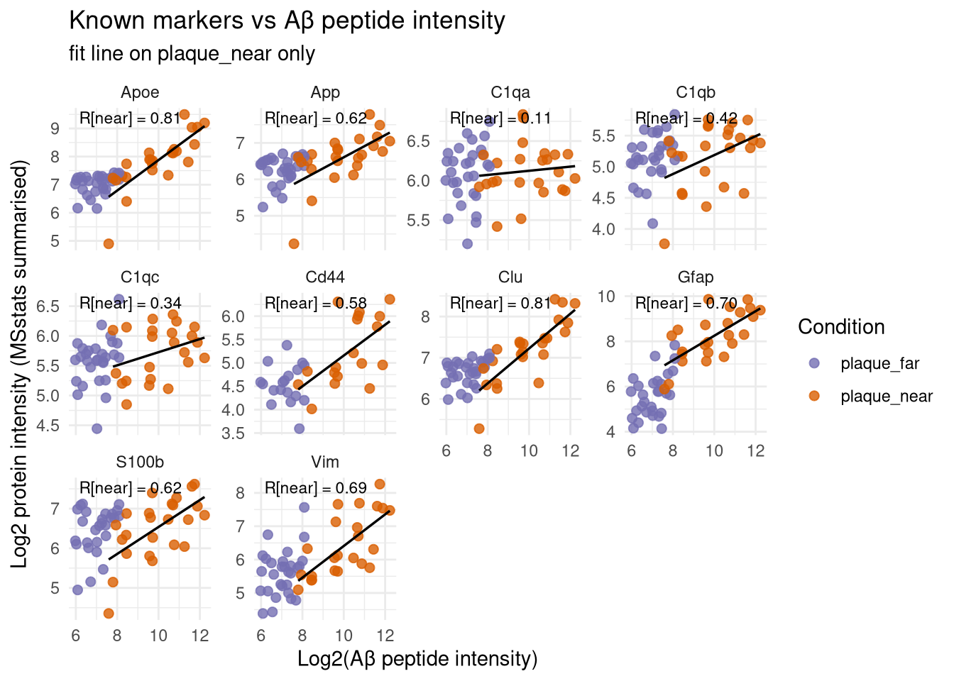

Code

ggsave(file.path(graphs_dir, "ab_marker_scatter.pdf"),
       width = 12, height = 9)

`geom_smooth()` using formula = 'y ~ x'

Warning: Removed 8 rows containing non-finite outside the scale range (`stat_smooth()`).
Removed 21 rows containing missing values or values outside the scale range
(`geom_point()`).

Warning in grid.Call.graphics(C_text, as.graphicsAnnot(x$label), x$x, x$y, :
conversion failure on 'Log2(Aβ peptide intensity)' in 'mbcsToSbcs': for β
(U+03B2)

Warning in grid.Call.graphics(C_text, as.graphicsAnnot(x$label), x$x, x$y, :
conversion failure on 'Known markers vs Aβ peptide intensity' in 'mbcsToSbcs':
for β (U+03B2)

Session info

Code

sessionInfo()

R version 4.5.1 (2025-06-13)
Platform: x86_64-pc-linux-gnu
Running under: Rocky Linux 8.7 (Green Obsidian)

Matrix products: default
BLAS/LAPACK: FlexiBLAS OPENBLAS;  LAPACK version 3.12.0

locale:
 [1] LC_CTYPE=en_GB.UTF-8       LC_NUMERIC=C              
 [3] LC_TIME=en_GB.UTF-8        LC_COLLATE=en_GB.UTF-8    
 [5] LC_MONETARY=en_GB.UTF-8    LC_MESSAGES=en_GB.UTF-8   
 [7] LC_PAPER=en_GB.UTF-8       LC_NAME=C                 
 [9] LC_ADDRESS=C               LC_TELEPHONE=C            
[11] LC_MEASUREMENT=en_GB.UTF-8 LC_IDENTIFICATION=C       

time zone: Europe/London
tzcode source: system (glibc)

attached base packages:
[1] stats     graphics  grDevices utils     datasets  methods   base     

other attached packages:
[1] purrr_1.2.1         ggrepel_0.9.6       ggplot2_4.0.2      
[4] tibble_3.3.1        tidyr_1.3.2         dplyr_1.2.0        
[7] qs2_0.1.6           data.table_1.18.2.1

loaded via a namespace (and not attached):
 [1] Matrix_1.7-4          gtable_0.3.6          jsonlite_2.0.0       
 [4] compiler_4.5.1        tidyselect_1.2.1      Rcpp_1.1.1           
 [7] splines_4.5.1         textshaping_1.0.3     systemfonts_1.3.1    
[10] scales_1.4.0          yaml_2.3.12           fastmap_1.2.0        
[13] lattice_0.22-7        R6_2.6.1              labeling_0.4.3       
[16] generics_0.1.4        knitr_1.51            htmlwidgets_1.6.4    
[19] stringfish_0.17.0     pillar_1.11.1         RColorBrewer_1.1-3   
[22] rlang_1.1.7           xfun_0.56             S7_0.2.1             
[25] RcppParallel_5.1.11-1 otel_0.2.0            cli_3.6.5            
[28] mgcv_1.9-4            withr_3.0.2           magrittr_2.0.4       
[31] digest_0.6.39         grid_4.5.1            nlme_3.1-168         
[34] lifecycle_1.0.5       vctrs_0.7.1           evaluate_1.0.5       
[37] glue_1.8.0            farver_2.1.2          ragg_1.5.0           
[40] rmarkdown_2.30        tools_4.5.1           pkgconfig_2.0.3      
[43] htmltools_0.5.9