6. Concordance between limma and MSstats

==================================================================

MSstats vs limma Concordance Analysis

Author: Carlo Zanetti

This script evaluates the consistency between MSstats and limma. It merges results from both methods to identify shared biological signals and pipeline specific differences.

Workflow overview

Data loading and visualisation

Import Msstats and limma data
Gene mapping and Annotation

Only necessary for Msstats
Thresholding and categorisation

Apply significance cut-offs (FDR <0.05, |log2FC| > 0.5)
Concordance analysis

Calculate pearson correlation between log2FC values of the 2 pipelines for each comparison
Visualisation

Plots concordance scatter plots between each pipeline and comparison.

Labels top 30 most highly changed genes using ggrepel

Produces tables summarising detction overlap and pipeline-specific abundant proteins

==================================================================

Load libraries

Code

suppressPackageStartupMessages({
library(data.table)
library(qs2)
library(dplyr)
library(ggplot2)
library(ggrepel)
library(purrr)
library(stringr)
library(clusterProfiler)
library(org.Mm.eg.db)
library(enrichplot)
library(ggVennDiagram)
})

Read in limma and msstats objects

Code

base_dir <- "/nemo/lab/destrooperb/home/shared/zanettc/millie_proteomics"
run_num <- "run5"
results_dir <- file.path(base_dir, "results", run_num)

objects_dir <- file.path(base_dir, "data", "processed", run_num)
millie_dir <- file.path(base_dir, "data", "processed_millie")
graphs_dir <- file.path(results_dir, "concordance")


millie_f_v_c <- read.csv(file.path(millie_dir, "limma_all_proteins_Plaque_far_vs_Control.csv"))
millie_n_v_c <- read.csv(file.path(millie_dir, "limma_all_proteins_Plaque_near_vs_Control.csv"))
millie_n_v_f <- read.csv(file.path(millie_dir, "limma_all_proteins_Plaque_near_vs_Far.csv"))

res_df <- fread(file.path(results_dir, "Full_GroupComparison_Results.csv"))
clean_spec_raw <- fread(file.path(base_dir, "data/processed/run1/clean_spec_raw.csv"))

Convert msstats to gene names

Code

protein_dictionary <- clean_spec_raw %>%
  dplyr::select(Protein = PG.ProteinGroups, 
         Gene = PG.Genes, 
         Description = PG.ProteinDescriptions) %>%
  distinct()

msstats_ready <- res_df %>%
  # Filter for your specific comparison (Label) and handle NAs
  filter(!is.na(adj.pvalue), is.finite(log2FC)) %>%
  
  # Join with dictionary
  left_join(protein_dictionary, by = "Protein") %>%
  
  # Clean up Gene names and define significance
  mutate(
    # Fallback to Protein ID if Gene name is missing or empty
    Gene = ifelse(is.na(Gene) | Gene == "", Protein, Gene),
    
    # Define significance categories
    Status = case_when(
      adj.pvalue < 0.05 & log2FC > 0.5 ~ "Upregulated",
      adj.pvalue < 0.05 & log2FC < -0.5 ~ "Downregulated",
      TRUE ~ "Not Significant"
    )
  ) %>%
  
  # Ranking for plotting/reporting
  group_by(Label, Status) %>%
  mutate(Rank = rank(adj.pvalue, ties.method = "first")) %>%
  ungroup()


msstats_ready %>% 
  filter(Label == "PlaqueNear_vs_PlaqueFar") %>%
  filter(log2FC > 0.5 & adj.pvalue < 0.05)

Combine millie’s dataframes into a mega merged one

Code

# Add labels to Millie's data to match MSstats 'Label' names
# Check your msstats_ready$Label to ensure these strings match exactly!
millie_combined <- bind_rows(
  millie_f_v_c %>% mutate(Label = "PlaqueFar_vs_Control"),
  millie_n_v_c %>% mutate(Label = "PlaqueNear_vs_Control"),
  millie_n_v_f %>% mutate(Label = "PlaqueNear_vs_PlaqueFar")
) %>%
dplyr::rename(
  log2FC_limma = logFC,
  adj.pvalue_limma = adj.P.Val
) %>%
mutate(
  Status_limma = case_when(
    adj.pvalue_limma < 0.05 & log2FC_limma > 0.5 ~ "Upregulated",
    adj.pvalue_limma < 0.05 & log2FC_limma < -0.5 ~ "Downregulated",
    TRUE ~ "Not Significant"
  )
) %>%
dplyr::select(Gene, Label, log2FC_limma, adj.pvalue_limma, Status_limma)

millie_combined

Code

write.csv(millie_combined, file.path(millie_dir, "millie_combined.csv"))

combine both msstats and limma dataframes

Code

comparison_df <- msstats_ready %>%
  dplyr::select(Protein, Gene, Label, log2FC_msstats = log2FC, adj.pvalue_msstats = adj.pvalue, Status_msstats = Status) %>%
  full_join(millie_combined, by = c("Gene", "Label")) %>%
  mutate(
    # Create a column to easily find discrepancies
    Agreement = case_when(
      Status_msstats == Status_limma ~ "Consistent",
      Status_msstats == "Not Significant" | Status_limma == "Not Significant" ~ "Pipeline Specific",
      TRUE ~ "Contradictory" # One says Up, one says Down
    )
  )

# Preview the overlap
table(comparison_df$Status_msstats, comparison_df$Status_limma)

                 
                  Downregulated Not Significant Upregulated
  Downregulated               3              15           0
  Not Significant            25           15587          33
  Upregulated                 0             645         177

Code

comparison_df %>% filter(Gene== "Cd44")

Plot concordance results

Code

plot_data <- comparison_df %>%
  # 1. Determine Significance categories based on your previous Status columns
  mutate(
    Significance = case_when(
      Status_msstats != "Not Significant" & Status_limma != "Not Significant" ~ "Significant in Both",
      Status_msstats != "Not Significant" & Status_limma == "Not Significant" ~ "Significant in MSstats only",
      Status_msstats == "Not Significant" & Status_limma != "Not Significant" ~ "Significant in limma only",
      TRUE ~ "Not Significant"
    ),
    # 2. Calculate distance from origin (Magnitude in both) to pick top labels
    # Using coalesce to handle NAs just in case a protein is only in one pipeline
    dist = sqrt(coalesce(log2FC_msstats, 0)^2 + coalesce(log2FC_limma, 0)^2)
  )

# Define your colors to match the exact spelling of categories
sig_colors <- c(
  "Significant in Both"         = "purple",
  "Significant in MSstats only" = "#00BFC4", # Cyan/Blue
  "Significant in limma only"   = "#F8766D", # Coral/Red
  "Not Significant"             = "grey80"
)

# --- STEP 2: Loop through each comparison and plot ---
comparisons <- unique(plot_data$Label)

for (comp in comparisons) {
  
  cat("Plotting:", comp, "\n")
  
  # Subset data for the current comparison
  df_sub <- plot_data %>% filter(Label == comp)
  
  # Check if we have data to plot before proceeding
  if(nrow(df_sub %>% filter(!is.na(log2FC_msstats) & !is.na(log2FC_limma))) == 0) {
    message(paste("No overlapping data found for:", comp, "- skipping."))
    next 
  }
  
  # Get top 30 genes to label based on distance from origin
  genes_to_label <- df_sub %>%
    filter(Significance != "Not Significant") %>%
    slice_max(order_by = dist, n = 30, with_ties = FALSE)
  
  # Calculate Pearson correlation for the subtitle 
  cor_val <- round(cor(df_sub$log2FC_msstats, df_sub$log2FC_limma, use = "complete.obs"), 3)
  
  # Clean up the comparison name for the plot title (e.g., "PlaqueNear_vs_Control" -> "Plaque Near vs Control")
  clean_title <- gsub("_", " ", comp)
  # Optional: Add spaces before capital letters if your label is CamelCase
  # clean_title <- gsub("([a-z])([A-Z])", "\\1 \\2", clean_title) 
  
  
  #### settings to make plot look pretty -> so all genes fit nicely in plot
  x_bulk <- quantile(df_sub$log2FC_limma, probs = c(0.01, 0.99), na.rm = TRUE)
  y_bulk <- quantile(df_sub$log2FC_msstats, probs = c(0.01, 0.99), na.rm = TRUE)
  
  #Get the range of the proteins we actually want to label
  x_label_range <- range(genes_to_label$log2FC_limma, na.rm = TRUE)
  y_label_range <- range(genes_to_label$log2FC_msstats, na.rm = TRUE)
  
  # 3. Final Limits: Use the wider of the two ranges so labels aren't cut off
  final_xlim <- c(min(x_bulk[1], x_label_range[1]), max(x_bulk[2], x_label_range[2]))
  final_ylim <- c(min(y_bulk[1], y_label_range[1]), max(y_bulk[2], y_label_range[2]))
  
  # Add 15% padding so labels have room to "repel" into
  x_pad <- diff(final_xlim) * 0.15
  y_pad <- diff(final_ylim) * 0.15
  
  
  
  # Build The Plot
  p <- ggplot(df_sub, aes(x = log2FC_limma, y = log2FC_msstats)) +
    
    # 1. Diagonal and Axes
    geom_abline(slope = 1, intercept = 0, color = "red", linetype = "solid", linewidth = 0.5) +
    geom_hline(yintercept = 0, linetype = "dashed", color = "grey50") +
    geom_vline(xintercept = 0, linetype = "dashed", color = "grey50") +
    
    # 2. Scatter Points
    geom_point(aes(color = Significance), alpha = 0.6, size = 2) +
    
    # 3. Optimized Labels (Mapped to your "Gene" column)
    geom_label_repel(
      data = genes_to_label, 
      aes(label = Gene, color = Significance),
      size = 4,                  
      fontface = "bold",         
      box.padding = 0.5,         
      point.padding = 0.3,       
      force = 2,                 
      max.overlaps = Inf,        
      min.segment.length = 0,    
      show.legend = FALSE,
      fill = "white"
    ) +
    
    # 4. Styling
    scale_color_manual(values = sig_colors) +
    coord_cartesian(
      xlim = c(final_xlim[1] - x_pad, final_xlim[2] + x_pad),
      ylim = c(final_ylim[1] - y_pad, final_ylim[2] + y_pad),
      expand = FALSE # Keeps our manual padding exact
    ) + 
    theme_bw(base_size = 16) + 
    
    labs(
      title = paste("Concordance:", clean_title),
      subtitle = paste("limma vs. MSstats | Pearson r =", cor_val),
      x = "limma Log2FC",
      y = "MSstats Log2FC",
      color = "Significance (FDR < 0.05)"
    ) +
    
    theme(
      legend.position = "bottom",
      legend.text = element_text(size = 12),
      legend.title = element_text(size = 12, face = "bold"),
      panel.grid.minor = element_blank(),
      plot.title = element_text(face = "bold", size = 18),
      axis.title = element_text(face = "bold")
    ) + 
    guides(color = guide_legend(
      override.aes = list(size = 5), 
      nrow = 2
    ))
  
  # Print to RStudio viewer/console so you can see them as they generate
  print(p)
  
  # Sanitize filename (replace spaces/special chars with underscores)
  safe_filename <- str_replace_all(comp, "[^A-Za-z0-9]+", "_")
  safe_filename <- str_replace(safe_filename, "_$", "")
  
  # Save to PDF
  ggsave(
    filename = file.path(graphs_dir, paste0("MSstats_vs_limma_concordance_", safe_filename, ".pdf")),
    plot = p,
    width = 10,
    height = 10,
    dpi = 300
  )
}

Plotting: PlaqueNear_vs_Control

Warning: Removed 222 rows containing missing values or values outside the scale range
(`geom_point()`).
Removed 222 rows containing missing values or values outside the scale range
(`geom_point()`).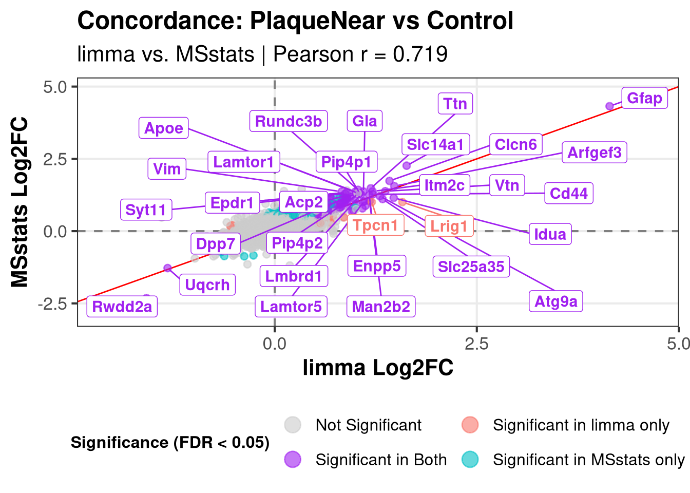

Plotting: PlaqueFar_vs_Control

Warning: Removed 222 rows containing missing values or values outside the scale range
(`geom_point()`).
Removed 222 rows containing missing values or values outside the scale range
(`geom_point()`).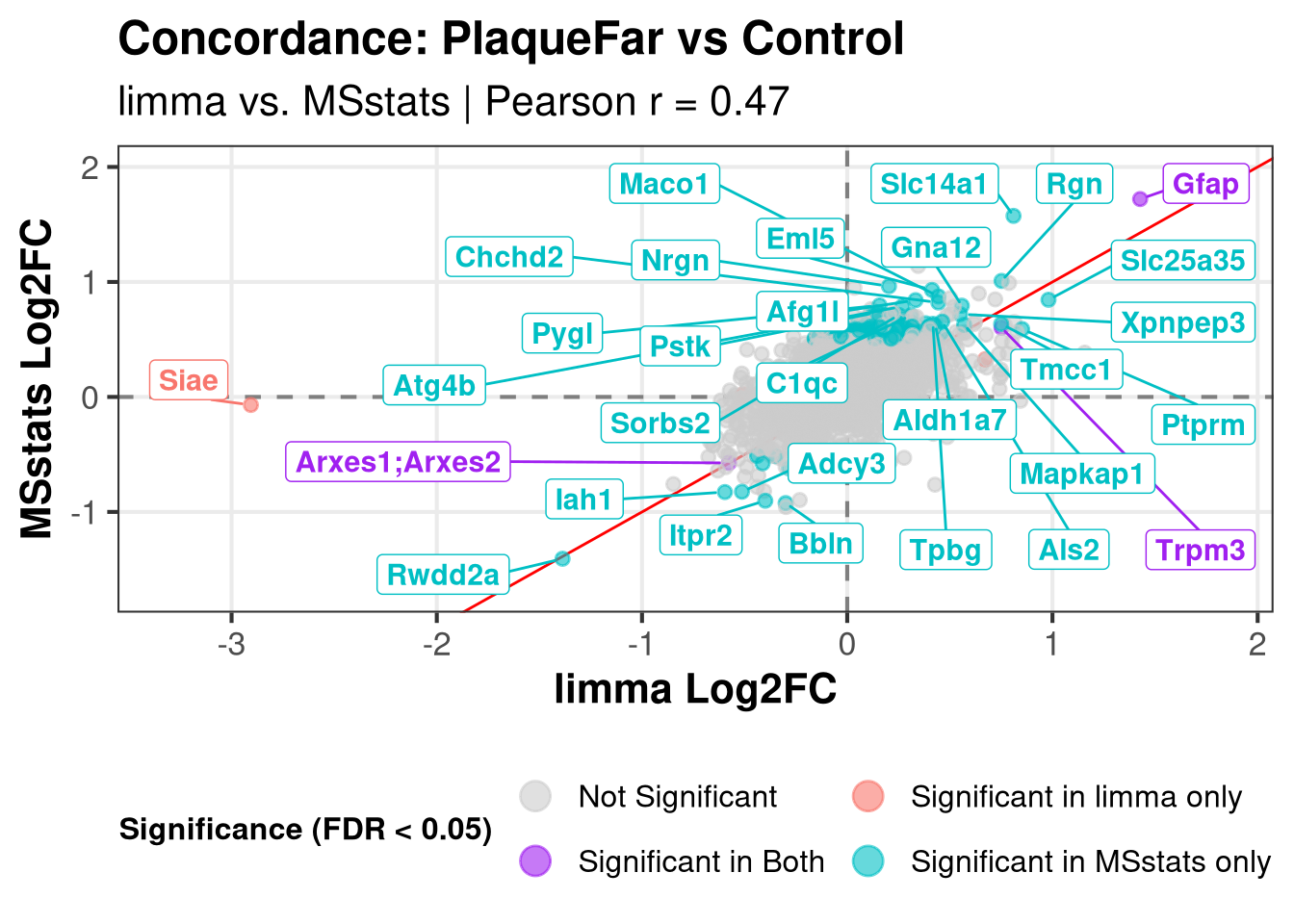

Plotting: PlaqueNear_vs_PlaqueFar

Warning: Removed 221 rows containing missing values or values outside the scale range
(`geom_point()`).

Warning: Removed 221 rows containing missing values or values outside the scale range
(`geom_point()`).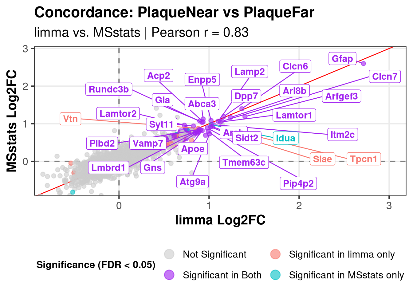

Code

cat("All plots generated and saved successfully to:", graphs_dir, "\n")

All plots generated and saved successfully to: /nemo/lab/destrooperb/home/shared/zanettc/millie_proteomics/results/run5/concordance

Print summary table comparing the two methods

Summarises the overlap in detection and significance.

Code

summary_table <- comparison_df %>%
  group_by(Label) %>%
  summarise(
    # 1. Total Detected overall (union of both methods)
    Total_Detected_Overall = n(),
    
    # 2. Detected by specific methods
    Detected_MSstats = sum(!is.na(log2FC_msstats)),
    Detected_limma   = sum(!is.na(log2FC_limma)),
    
    # 3. Both Detected (Shared column)
    Both_Detected    = sum(!is.na(log2FC_msstats) & !is.na(log2FC_limma)),
    
    # 4. Significant (FDR < 0.05)
    Sig_MSstats      = sum(Status_msstats != "Not Significant", na.rm = TRUE),
    Sig_limma        = sum(Status_limma != "Not Significant", na.rm = TRUE),
    
    # 5. Both Significant (Shared column)
    Both_Significant = sum(Status_msstats != "Not Significant" & 
                           Status_limma != "Not Significant", na.rm = TRUE)
  ) %>%
  # Clean up the Label for readability
  mutate(Label = gsub("_", " ", Label))

summary_table

How many signficant proteins from MSstats pipeline did the limma pipeline detect as present?

Code

#Filter for signficant msstats proteins and check if detected by Millie
msstats_sig_analysis <- comparison_df %>%
  filter(Status_msstats != "Not Significant") %>%
  mutate(
    Detected_by_Millie = ifelse(!is.na(log2FC_limma), "Yes", "No")
  )

# Summarize the findings per comparison
detection_overlap <- msstats_sig_analysis %>%
  group_by(Label, Detected_by_Millie) %>%
  tally(name = "Protein_Count") %>%
  tidyr::pivot_wider(names_from = Detected_by_Millie, values_from = Protein_Count, names_prefix = "Detected_by_limma_")

print(detection_overlap)

# A tibble: 3 × 3
# Groups:   Label [3]
  Label                   Detected_by_limma_No Detected_by_limma_Yes
  <chr>                                  <int>                 <int>
1 PlaqueFar_vs_Control                       3                   310
2 PlaqueNear_vs_Control                      4                   455
3 PlaqueNear_vs_PlaqueFar                   NA                    74

What were the signficant proteins that were detected in the limma analysis but not msstats?

Code

limma_exclusive_sig <- comparison_df %>%
  filter(Label == "PlaqueNear_vs_PlaqueFar") %>%
  filter(Status_limma != "Not Significant" & Status_msstats == "Not Significant") %>%
  dplyr::select(Gene, 
         log2FC_limma, adj.pvalue_limma, 
         log2FC_msstats, adj.pvalue_msstats) %>%
  arrange(adj.pvalue_limma)

limma_exclusive_sig

What were the signficant proteins that were detected in the msstats analysis but not limma?

Code

msstats_exclusive_sig <- comparison_df %>%
  filter(Label == "PlaqueNear_vs_PlaqueFar") %>%
  filter(Status_limma == "Not Significant" & Status_msstats != "Not Significant") %>%
  dplyr::select(Gene, 
         log2FC_limma, adj.pvalue_limma, 
         log2FC_msstats, adj.pvalue_msstats) %>%
  arrange(adj.pvalue_limma)

msstats_exclusive_sig

Check for how many MSstats proteins were FDR <0.05 but < 0.5 log2FC

Code

check_cutoffs_msstats <- comparison_df %>%
  filter(Label == "PlaqueNear_vs_PlaqueFar") %>%
  filter(adj.pvalue_msstats < 0.05 & Status_msstats == "Not Significant") %>%
  dplyr::select(Gene, log2FC_msstats, adj.pvalue_msstats)

check_cutoffs_msstats

Check for how many limma proteins were FDR <0.05 but < 0.5 log2FC

Code

check_cutoffs_limma <- comparison_df %>%
  filter(Label == "PlaqueNear_vs_PlaqueFar") %>%
  filter(adj.pvalue_msstats < 0.05 & Status_limma == "Not Significant") %>%
  dplyr::select(Gene, log2FC_limma, adj.pvalue_limma, log2FC_msstats, adj.pvalue_msstats)

check_cutoffs_limma

Identify genes that are up in both plaque distances

Code

# 1. Isolate significant genes for Near vs Control (MSstats)
near_vs_control_sig <- comparison_df %>%
  filter(Label == "PlaqueNear_vs_Control" & Status_msstats != "Not Significant") %>%
  pull(Gene) %>%
  unique()

# 2. Isolate significant genes for Far vs Control (MSstats)
far_vs_control_sig <- comparison_df %>%
  filter(Label == "PlaqueFar_vs_Control" & Status_msstats != "Not Significant") %>%
  pull(Gene) %>%
  unique()

# 3. Calculate intersections and differences
shared_msstats_genes <- intersect(near_vs_control_sig, far_vs_control_sig)
unique_to_near <- setdiff(near_vs_control_sig, far_vs_control_sig)
unique_to_far <- setdiff(far_vs_control_sig, near_vs_control_sig)

cat("MSstats Significance Overlap Summary:\n")

MSstats Significance Overlap Summary:

Code

cat("-------------------------------------\n")

-------------------------------------

Code

cat("Total Significant in Near vs Control:", length(near_vs_control_sig), "\n")

Total Significant in Near vs Control: 459

Code

cat("Total Significant in Far vs Control:", length(far_vs_control_sig), "\n")

Total Significant in Far vs Control: 313

Code

cat("Shared between both (Intersection):", length(shared_msstats_genes), "\n")

Shared between both (Intersection): 137

Code

cat("Unique to Near vs Control:", length(unique_to_near), "\n")

Unique to Near vs Control: 322

Code

cat("Unique to Far vs Control:", length(unique_to_far), "\n\n")

Unique to Far vs Control: 176

Plot on venn diagram genes that are up in both plaque distances

Code

# 1. Group the significant gene lists into a named list
msstats_venn_list <- list(
  "Near vs Control" = near_vs_control_sig,
  "Far vs Control"  = far_vs_control_sig
)

# 2. Generate the Venn Diagram
venn_plot <- ggVennDiagram(msstats_venn_list, 
                           label_alpha = 0, 
                           set_color = "black",
                           label = "both") + # Shows count and percentage
  scale_fill_gradient(low = "white", high = "#00BFC4") + 
  theme_void(base_size = 14) +
  labs(title = "MSstats: Significant Proteins Overlap", fill = "Gene Count") +
  theme(
    plot.title = element_text(face = "bold", hjust = 0.5),
    # Add large margins (Top, Right, Bottom, Left) to prevent label clipping
    plot.margin = margin(20, 60, 20, 60) 
  ) +
  # This allows labels to draw outside the "official" plot area
  coord_cartesian(clip = "off")

Coordinate system already present.
ℹ Adding new coordinate system, which will replace the existing one.

Code

# Print the plot
print(venn_plot)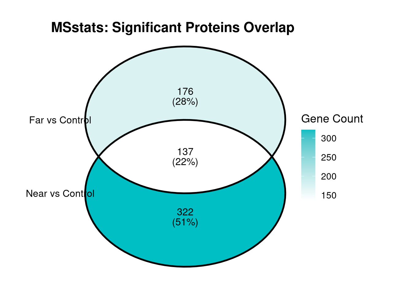

Code

# 4. Save the plot to your graphs directory
ggsave(
  filename = file.path(graphs_dir, "MSstats_Near_vs_Far_Venn.pdf"),
  plot = venn_plot,
  width = 8,
  height = 6,
  dpi = 300
)

Far vs control only

Code

msstats_far_only_df <- comparison_df %>%
  filter(Label == "PlaqueFar_vs_Control") %>%
  filter(Gene %in% unique_to_far) %>%
  dplyr::select(Gene, log2FC_msstats, adj.pvalue_msstats, Status_msstats) %>%
  arrange(adj.pvalue_msstats)

# 2. Preview the top of the list
cat("Top 10 proteins unique to Plaque Far vs Control (MSstats):\n")

Top 10 proteins unique to Plaque Far vs Control (MSstats):

Code

msstats_far_only_df

Code

fwrite(msstats_far_only_df, file.path(results_dir, "msstats_plaque_far_vs_control_only.csv"))