Code
suppressPackageStartupMessages({
library(data.table)
library(qs2)
library(ggrepel)
library(ggplot2)
library(stringr)
library(glue)
library(dplyr)
library(msigdbr)
library(fgsea)
library(viridis)
library(readxl)
})==================================================================
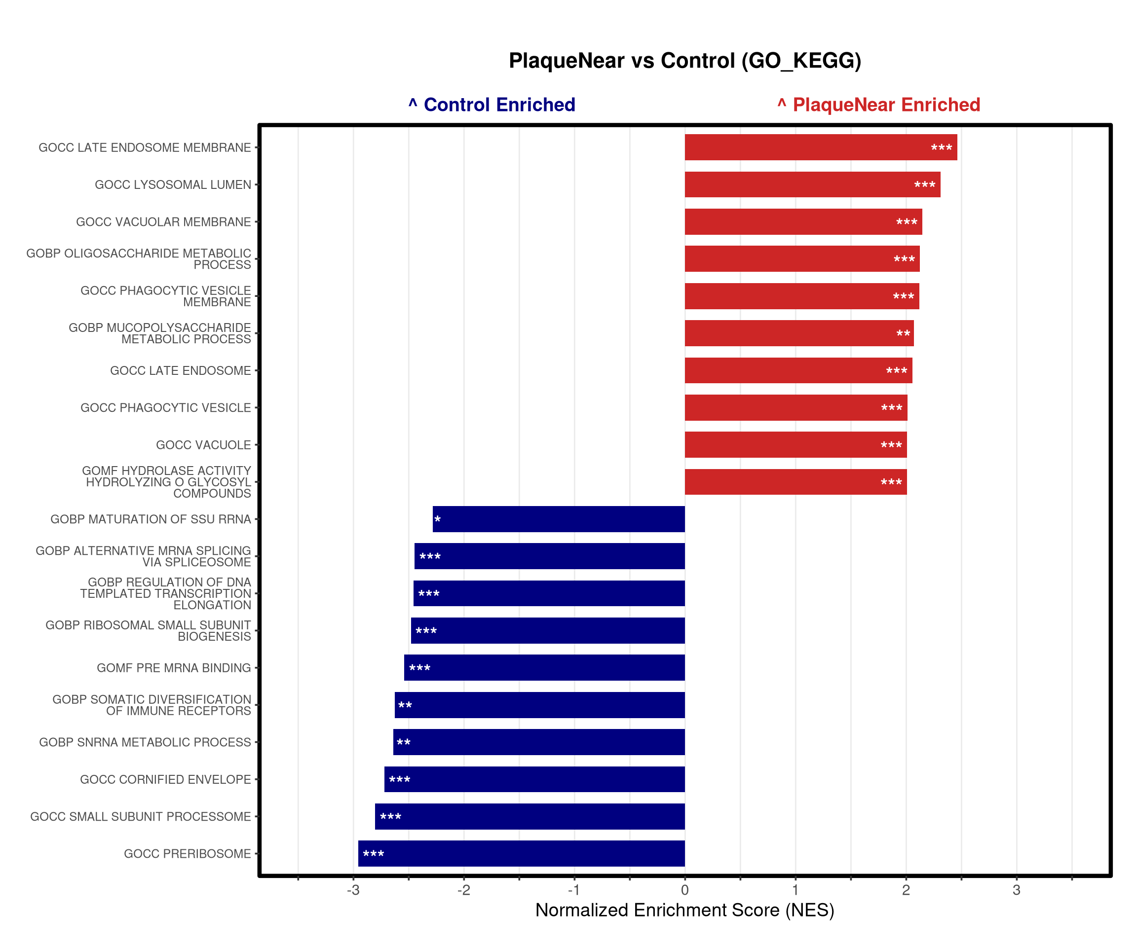
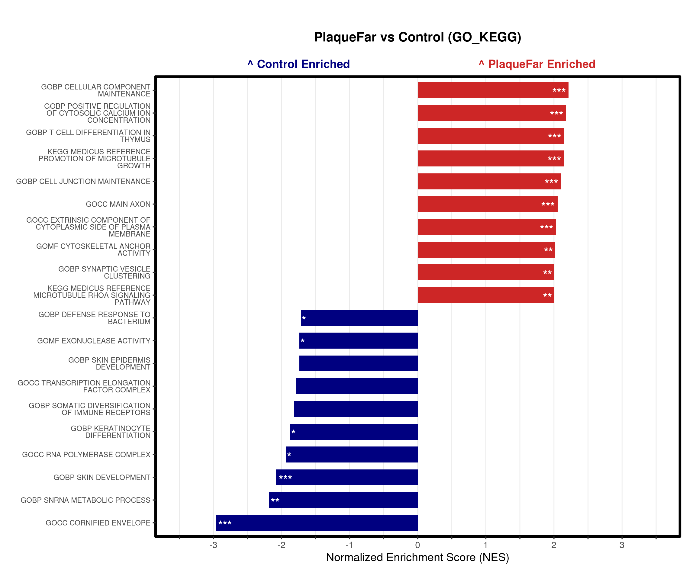
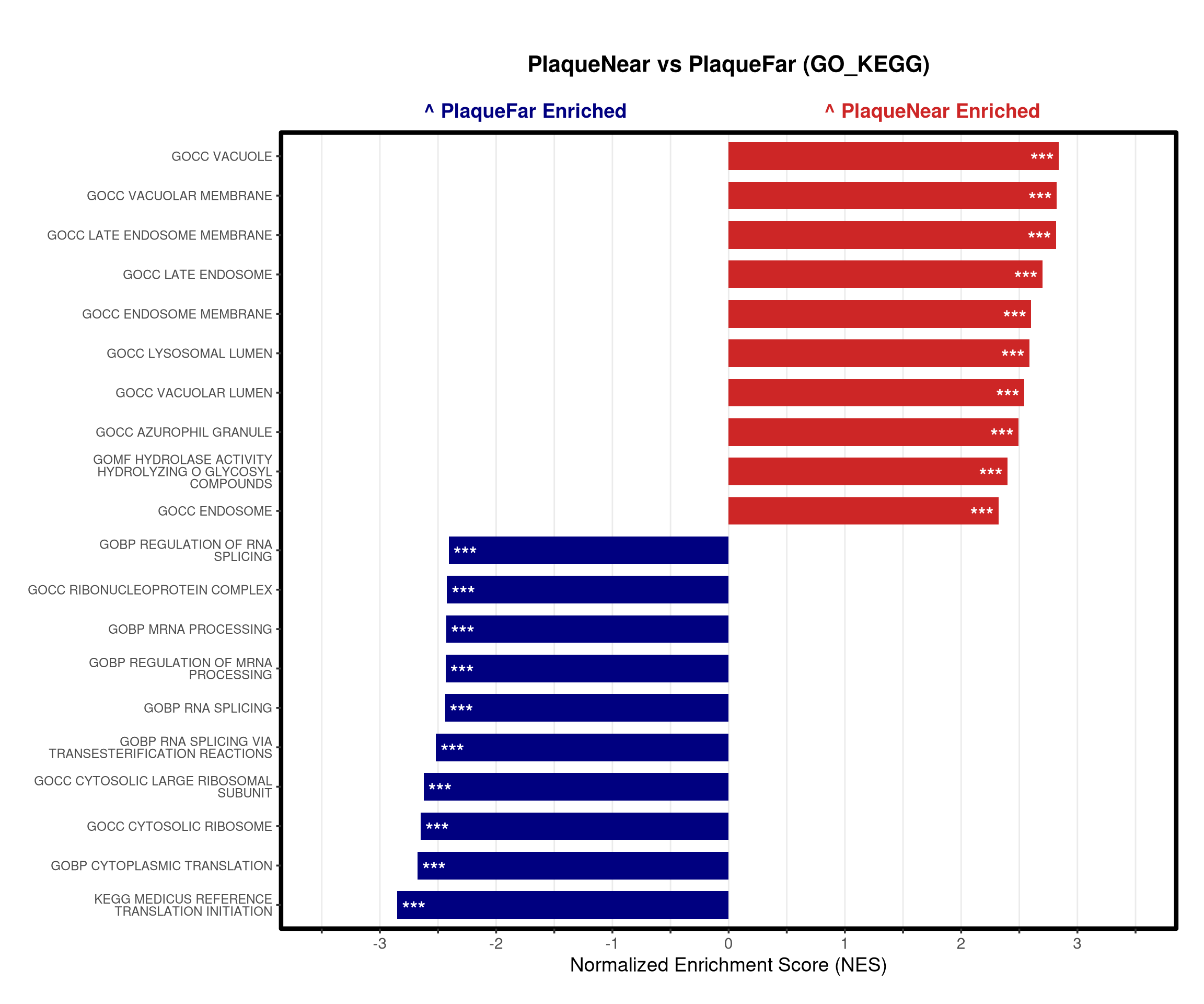
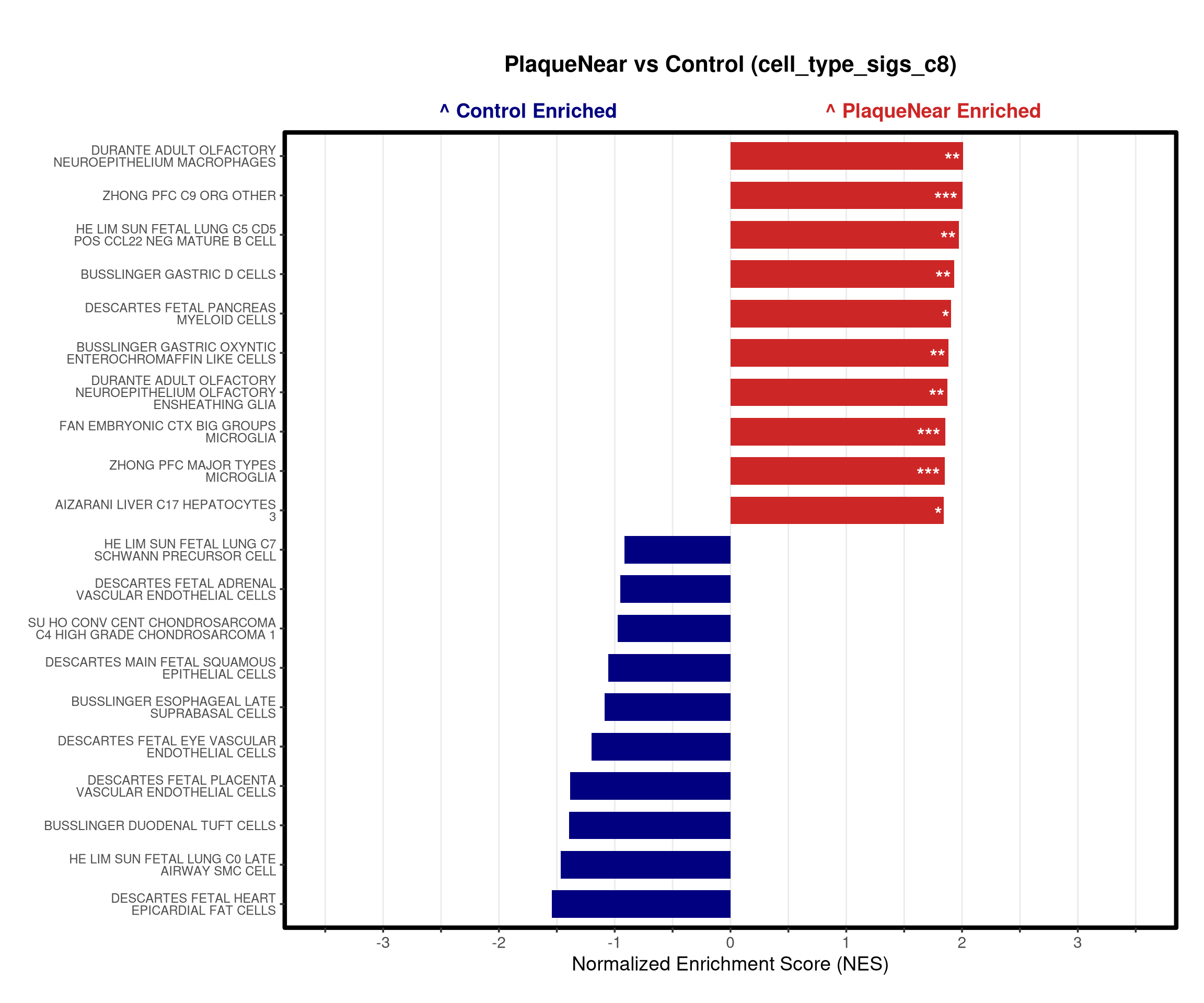
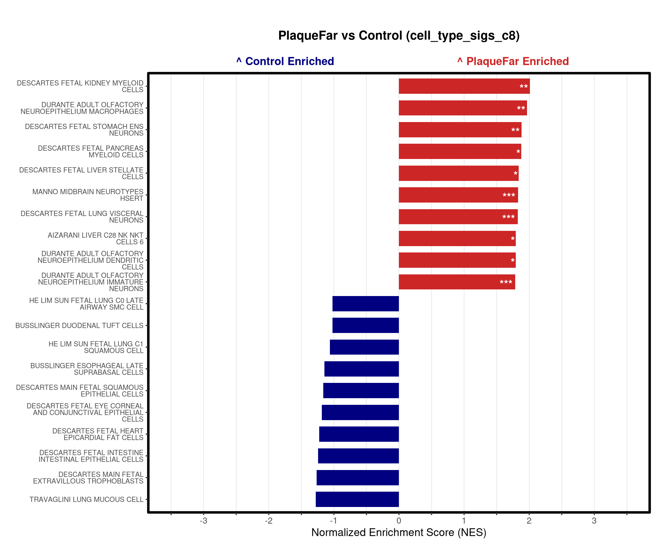
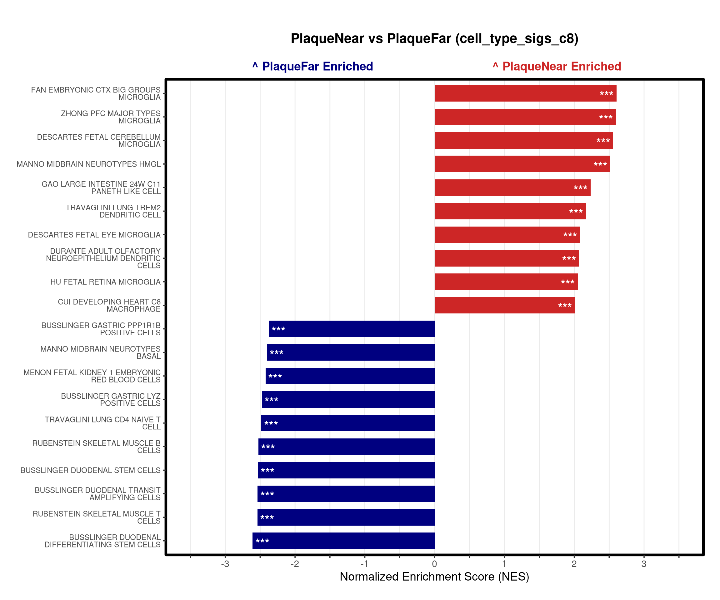
This script performs GSEA to identify biological pathways enriched in the differential expression lists generated by msstats. It uses the fgsea package.
1. Data Loading: Imports DE tables (CSV) from the msstats step.
2. Gene Set Prep: Loads pathways from multiple sources (GO / KEGG / cell type signatures (C8)/ DAA signature)
3. Ranking: Ranks proteins by Log2FC for every comparison.
4. Analysis Loop: Runs GSEA for every combination of [Comparison x Gene Set Database].
5. Visualization:
==================================================================
suppressPackageStartupMessages({
library(data.table)
library(qs2)
library(ggrepel)
library(ggplot2)
library(stringr)
library(glue)
library(dplyr)
library(msigdbr)
library(fgsea)
library(viridis)
library(readxl)
})base_dir <- "/nemo/lab/destrooperb/home/shared/zanettc/millie_proteomics"
run_num <- "run5"
results_dir <- file.path(base_dir, "results", run_num)
objects_dir <- file.path(base_dir, "data", "processed", run_num)
raw_dir <- file.path(base_dir, "data", "raw")
dir.create(results_dir, recursive = TRUE, showWarnings = FALSE)
dir.create(objects_dir, recursive = TRUE, showWarnings = FALSE)
dir.create(raw_dir, recursive = TRUE, showWarnings = FALSE)#seurat <- qs_read(glue("output/{run_num}/objects/prelabelled_integrated_rpca.qs2"))
res_df <- fread(file.path(results_dir, "Full_GroupComparison_Results.csv"))
clean_spec_raw <- fread(file.path(base_dir, "data/processed/run1/clean_spec_raw.csv"))
protein_dictionary <- clean_spec_raw %>%
dplyr::select(Protein = PG.ProteinGroups,
Gene = PG.Genes,
Description = PG.ProteinDescriptions) %>%
distinct()
res_df# ==============================================================================
# 1. HELPER FUNCTIONS
# ==============================================================================
# A. Create Rank Vector from MSstats Data
prep_msstats_ranks <- function(msstats_res, dict, comp_label) {
df <- msstats_res %>%
filter(Label == comp_label) %>%
# Keep only finite log2FC values (removes Inf and -Inf)
filter(is.finite(log2FC)) %>%
left_join(dict, by = "Protein") %>%
filter(!is.na(Gene) & Gene != "") %>%
mutate(Gene = toupper(Gene)) %>%
mutate(adj.pvalue = ifelse(adj.pvalue == 0, 1e-300, adj.pvalue)) %>%
group_by(Gene) %>%
slice_max(order_by = abs(log2FC), n = 1, with_ties = FALSE) %>%
ungroup()
#rank by logFC
ranks <- df$log2FC
names(ranks) <- df$Gene
# Remove any unexpected NAs in names or values
ranks <- ranks[!is.na(ranks) & !is.na(names(ranks))]
return(sort(ranks, decreasing = TRUE))
}
# B. Core GSEA & Plotting Function
run_gsea_analysis <- function(ranks,
comparison_name,
geneset_name,
pathways,
base_objects_dir,
base_graphs_dir,
color_A = "firebrick3",
color_B = "navy") {
message(glue("Running GSEA | Set: {geneset_name} | Comp: {comparison_name}"))
# --- DYNAMIC LABEL GENERATION ---
# Split the comparison name to get the two groups (e.g., "PlaqueNear" and "PlaqueFar")
comp_parts <- str_split(comparison_name, "_vs_")[[1]]
if(length(comp_parts) == 2) {
group_A_label <- glue("{comp_parts[1]} Enriched") # Positive NES
group_B_label <- glue("{comp_parts[2]} Enriched") # Negative NES
} else {
group_A_label <- "Group A Enriched"
group_B_label <- "Group B Enriched"
}
# Clean title for the plot
clean_comp_title <- gsub("_", " ", comparison_name)
plot_title <- glue("{clean_comp_title} ({geneset_name})")
# --- Directories ---
current_objects_dir <- file.path(base_objects_dir, "GSEA_Analysis_logfc_x_pval", comparison_name)
current_graphs_dir <- file.path(base_graphs_dir, "GSEA_Analysis_logfc_x_pval", comparison_name)
dir.create(current_objects_dir, recursive = TRUE, showWarnings = FALSE)
dir.create(current_graphs_dir, recursive = TRUE, showWarnings = FALSE)
# --- Run FGSEA ---
pathways_upper <- lapply(pathways, toupper)
set.seed(42)
fgsea_res <- fgsea(
pathways = pathways_upper,
stats = ranks,
minSize = 15,
maxSize = 3000,
nproc = 4,
nPermSimple = 10000 #changed this
)
if (nrow(fgsea_res) == 0) {
warning(glue("No significant pathways for {geneset_name} in {comparison_name}"))
return(NULL)
}
# --- Tidy & Save ---
fgsea_res_tidy <- fgsea_res %>%
as_tibble() %>%
mutate(leadingEdge = sapply(leadingEdge, paste, collapse = ",")) %>%
mutate(pathway = gsub("_geneset", "", pathway)) %>%
arrange(padj)
write.csv(fgsea_res_tidy, file.path(current_objects_dir, glue("Table_{geneset_name}.csv")), row.names = FALSE)
# --- Barplot ---
top_gsea <- fgsea_res_tidy %>%
arrange(desc(NES)) %>%
slice_head(n = 10) %>%
bind_rows(fgsea_res_tidy %>% arrange(NES) %>% slice_head(n = 10)) %>%
distinct(pathway, .keep_all = TRUE) %>%
mutate(
sig_label = case_when(
padj < 0.001 ~ "***",
padj < 0.01 ~ "**",
padj < 0.05 ~ "*",
TRUE ~ ""
),
# Apply dynamic labels based on NES direction
fill_group = ifelse(NES > 0, group_A_label, group_B_label),
pathway = factor(pathway, levels = unique(pathway[order(NES)]))
)
if (nrow(top_gsea) == 0) return(fgsea_res_tidy)
axis_zoom <- 3.5
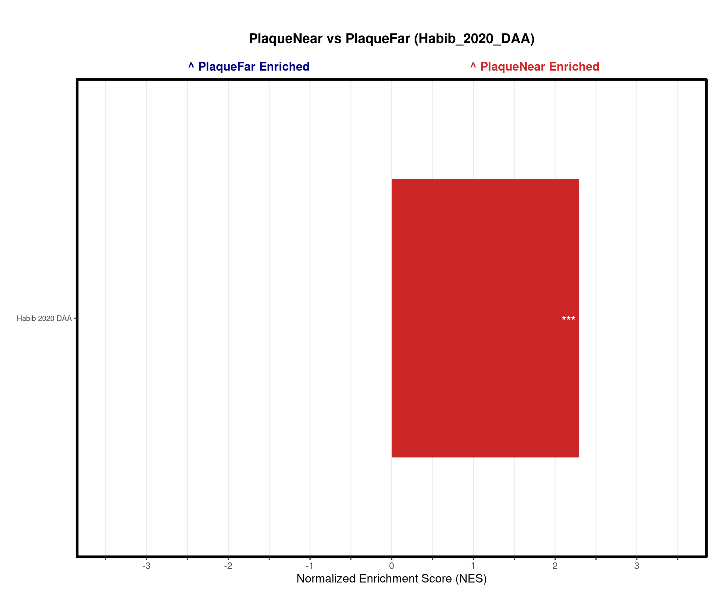
p_bar <- ggplot(top_gsea, aes(x = NES, y = pathway, fill = fill_group)) +
geom_col(width = 0.7) +
geom_text(aes(label = sig_label, hjust = ifelse(NES > 0, 1.2, -0.2)),
color = "white", size = 5, vjust = 0.75, fontface = "bold") +
scale_fill_manual(values = setNames(c(color_A, color_B), c(group_A_label, group_B_label))) +
scale_x_continuous(breaks = seq(-axis_zoom, axis_zoom, 0.5),
labels = function(x) ifelse(x %% 1 == 0, x, "")) +
labs(x = "Normalized Enrichment Score (NES)", y = NULL, title = plot_title) +
theme_bw(base_size = 14) +
theme(
panel.grid.major.x = element_line(color = "grey92", linewidth = 0.5),
panel.grid.major.y = element_blank(),
panel.grid.minor = element_blank(),
panel.border = element_rect(colour = "black", fill = NA, linewidth = 1.5),
legend.position = "none",
plot.title = element_text(hjust = 0.5, face = "bold", size = 16, margin = margin(b = 40)),
plot.margin = margin(t = 40, r = 20, b = 20, l = 20, unit = "pt"),
#ensure y axis has enough room, and tightens lines together
axis.text.y = element_text(size = 9, lineheight = 0.8)
) +
scale_y_discrete(labels = function(x) str_wrap(gsub("_", " ", x), width = 30)) +
# Dynamic text annotations at the top of the plot
annotate("text", x = -axis_zoom/2, y = Inf,
label = glue("^ {group_B_label}"), color = color_B, size = 5, fontface = "bold", vjust = -1.0) +
annotate("text", x = axis_zoom/2, y = Inf,
label = glue("^ {group_A_label}"), color = color_A, size = 5, fontface = "bold", vjust = -1.0) +
coord_cartesian(xlim = c(-axis_zoom, axis_zoom), clip = "off")
dyn_h <- 2 + (nrow(top_gsea) * 0.3)
dyn_w <- 5 + (max(nchar(as.character(top_gsea$pathway))) * 0.12)
print(p_bar)
ggsave(filename = file.path(current_graphs_dir, glue("Barplot_{geneset_name}.pdf")),
plot = p_bar, width = dyn_w, height = dyn_h, limitsize = FALSE)
# --- Dotplot (Top 10 Highest NES) ---
top_nes_gsea <- fgsea_res_tidy %>%
arrange(desc(NES)) %>%
slice_head(n = 10) %>%
mutate(pathway = factor(pathway, levels = unique(pathway[order(NES)])))
if (nrow(top_nes_gsea) > 0) {
# Define our wrap width
wrap_width <- 45
p_sig <- ggplot(top_nes_gsea, aes(x = NES, y = pathway, color = NES, size = -log10(padj))) +
geom_vline(xintercept = 0, linetype = "dashed", color = "grey60") +
geom_point(alpha = 0.8) +
scale_color_gradient2(low = color_B, mid = "grey90", high = color_A, midpoint = 0, name = "NES") +
scale_size_continuous(range = c(3, 8), name = "-log10(padj)") +
labs(x = "Normalized Enrichment Score (NES)", y = NULL,
title = glue("Top 10 Highest NES:\n{clean_comp_title} ({geneset_name})")) +
theme_bw(base_size = 14) +
theme(
panel.grid.major.x = element_line(color = "grey92", linewidth = 0.5),
panel.grid.major.y = element_line(color = "grey92", linewidth = 0.5, linetype = "dotted"),
panel.grid.minor = element_blank(),
panel.border = element_rect(colour = "black", fill = NA, linewidth = 1.5),
plot.title = element_text(hjust = 0.5, face = "bold", size = 14, margin = margin(b = 20)),
plot.margin = margin(t = 20, r = 10, b = 10, l = 10, unit = "pt"),
axis.text.y = element_text(lineheight = 0.8)
) +
scale_y_discrete(labels = function(x) str_wrap(gsub("_", " ", x), width = wrap_width))
# --- DYNAMIC SIZING ---
# Cap the character count at wrap_width so the plot doesn't stretch endlessly horizontally
max_chars <- min(max(nchar(as.character(top_nes_gsea$pathway))), wrap_width)
# Calculate dimensions: enough base room for the plot/legends + scaled room for text/points
dyn_h_sig <- 3 + (nrow(top_nes_gsea) * 0.4)
dyn_w_sig <- 4.5 + (max_chars * 0.1)
ggsave(filename = file.path(current_graphs_dir, glue("Dotplot_Top10_NES_{geneset_name}.pdf")),
plot = p_sig, width = dyn_w_sig, height = dyn_h_sig, limitsize = FALSE)
}
return(fgsea_res_tidy)
}# ==============================================================================
# 2. CONFIG & DATA LOADING
# ==============================================================================
GLOBAL_CONFIG <- list(
output_dir = file.path(results_dir, "GSEA_Results_Master"),
group_A = "Plaque Enriched",
group_B = "Control Enriched",
col_A = "firebrick3",
col_B = "navy"
)
# Load Gene Sets
#go and kegg sets
go_pathways <- gmtPathways("../../GO_human_all_genesets.gmt")
kegg_df <- msigdbr(species = "Mus musculus", collection = "C2", subcollection = "CP:KEGG_MEDICUS")Using human MSigDB with ortholog mapping to mouse. Use `db_species = "MM"` for mouse-native gene sets.
This message is displayed once per session.kegg_list <- split(x = kegg_df$gene_symbol, f = kegg_df$gs_name)
go_kegg_list <- c(go_pathways, kegg_list)
#cell type signature sets
c8_df <- msigdbr(species = "Mus musculus", category = "C8")Warning: The `category` argument of `msigdbr()` is deprecated as of msigdbr 10.0.0.
ℹ Please use the `collection` argument instead.c8_list <- split(x = c8_df$gene_symbol, f = c8_df$gs_name)
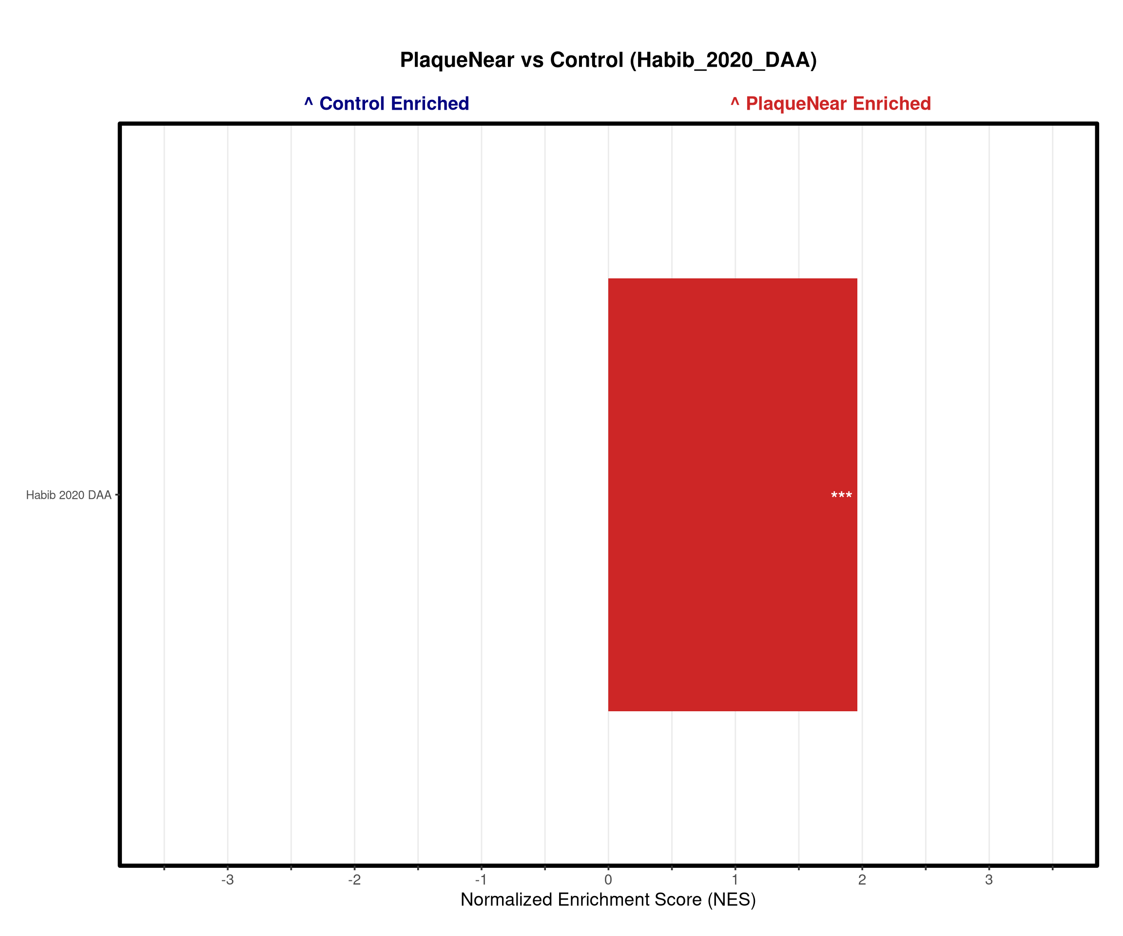
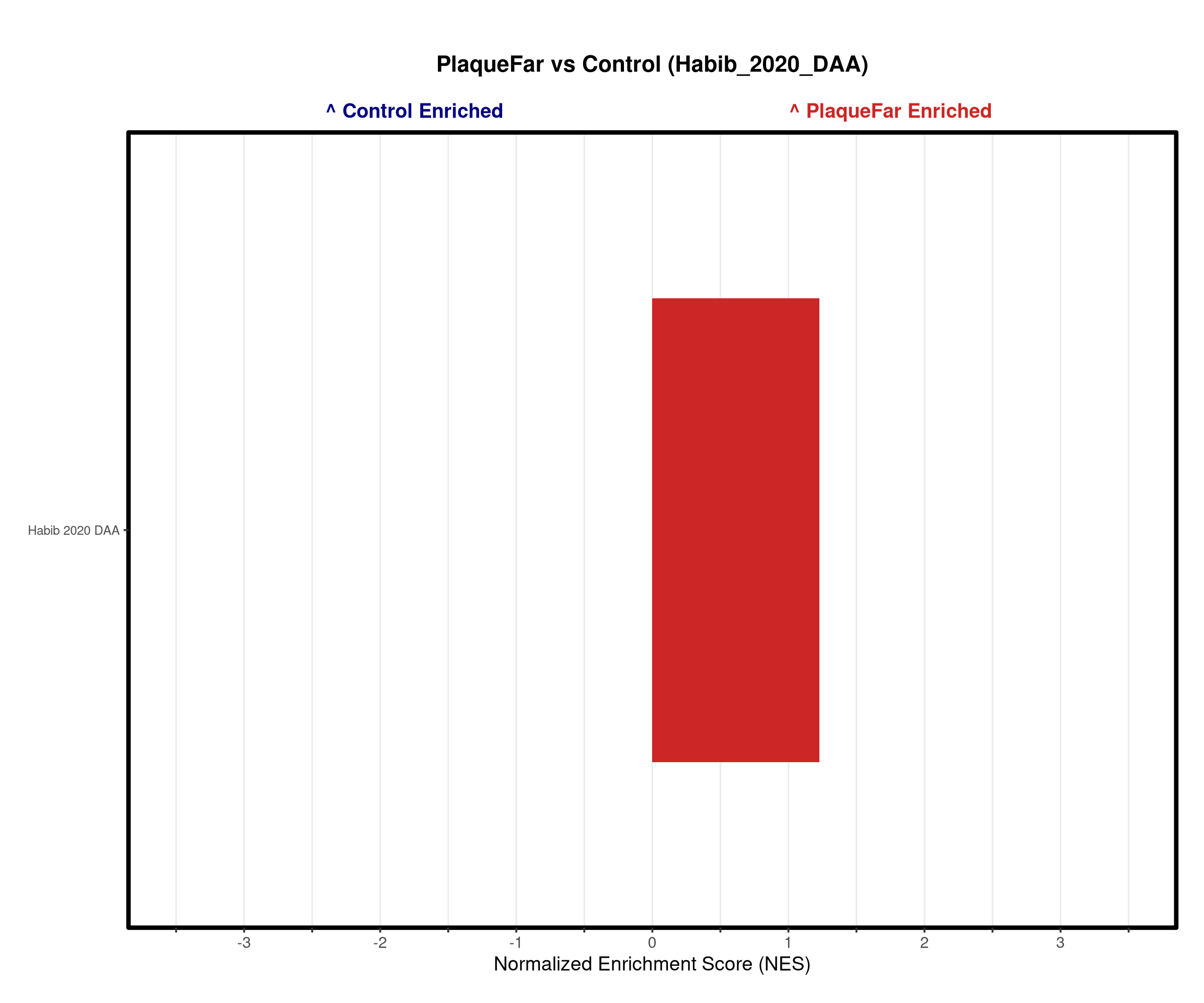
#DAA signature from from https://www.nature.com/articles/s41593-020-0624-8
daa_df <- read_excel(path = file.path(raw_dir, "DAA_Habib_2020.xlsx"), col_types = "text")
#Extract the genes as a character vector
daa_vector <- daa_df %>%
pull(Gene) %>%
toupper() %>%
unique()
daa_vector [1] "CST3" "APOE" "CLU" "GFAP"
[5] "CPE" "MT1" "CD81" "CD9"
[9] "MT2" "ID3" "CKB" "FXYD1"
[13] "VIM" "PRDX6" "CTSB" "CSMD1"
[17] "DBI" "FTH1" "HSD17B4" "ALDOC"
[21] "IGFBP5" "MLC1" "C4B" "NTRK2"
[25] "GSN" "KCNIP4" "GPM6B" "CNN3"
[29] "FTL1" "ATP1B2" "ID4" "PSAP"
[33] "PLCE1" "AQP4" "TAGLN3" "SORBS1"
[37] "TMEM47" "ITM2C" "SCD2" "ITM2B"
[41] "GPC5" "PRDX1" "CD63" "LAPTM4A"
[45] "LAMP1" "GSTM1" "TRPM3" "TSPAN3"
[49] "GPR37L1" "S100A6" "CTSD" "SPARC"
[53] "TMBIM6" "SCG3" "B2M" "NCAM2"
[57] "GM14964" "GGTA1" "ENOX1" "GLIS3"
[61] "S100A16" "TUBA1A" "CTSL" "S100B"
[65] "6330403K07RIK" "CHST2" "CHL1" "MATN4"
[69] "ANGPT1" "ADD3" "SERPINA3N" "TMEM176B"
[73] "ARHGEF4" "MGST1" "TUBB2B" "IFITM3"
[77] "GRM5" "ID2" "DHRS1" "SDC4"
[81] "OSMR" "CADPS" "LSAMP" "DST"
[85] "GADD45G" "THBS4" "DDR1" "SEMA6D"
[89] "RCN2" "CPNE8" "UBE2E2" "SELK"
[93] "SBNO2" "FBXO2" "TSC22D4" "SARAF"
[97] "TMEM176A" "PRKCA" "LAMP2" "ASPG"
[101] "MAN1A" "SLC38A1" "CAV2" "S100A1"
[105] "ABCA1" "CHIL1" "TST" "PRUNE2"
[109] "HIST1H2BC" "SLC3A2" "SYT11" "ERBB2IP"
[113] "GM10116" "KIF1A" "HRSP12" "SGCD"
[117] "STAT3" "LGALS1" "SLC16A1" "GPX4"
[121] "PDPN" "CD151" "USP53" "GRIK2"
[125] "PARD3B" "FXYD7" "FOS" "ID1"
[129] "CACNB2" "UBC" "PDIA4" "NKAIN2"
[133] "NRG2" "LXN" "HOPX" "SREBF1"
[137] "SLC35F1" "PDLIM4" "CEBPB" "CYR61"
[141] "SOX9" "SERPINF1" "NFKBIA" "NFE2L2"
[145] "SLC14A1" "ARHGAP6" "HSPA5" "SULF2"
[149] "NAALADL2" "TSPAN4" "NAV2" "CTNNBIP1"
[153] "BCAP31" "SLC39A14" "SHISA6" "APLP2"
[157] "SERPING1" "SPCS2" "EZR" "SCARB2"
[161] "RAB18" "GNAI2" "JUNB" "CLIC1"
[165] "PFKP" "HSPA2" "AEBP1" "IDH2"
[169] "PPIB" "ATRAID" "DGKI" "ATP6V0E"
[173] "JUND" "HNRNPK" "SULF1" "1700030F04RIK"
[177] "ITGB8" "MFAP3L" "S100A10" "NPC2"
[181] "SLC7A10" "REEP5" "VWA1" "SHISA5"
[185] "GM4876" "LGMN" "LGALS3BP" "GM3448"
[189] "TMCO1" "GM3764" "RAP1B" "TMEM59"
[193] "2810459M11RIK" "DEGS1" "EFCAB14" "1810058I24RIK"
[197] "GNA13" "SAMD4" "S1PR3" "MMP16"
[201] "HSD17B12" "SORBS2" "TUBB2A" "ATP6AP2"
[205] "KCNJ3" "RHOB" "NRG1" "EPDR1"
[209] "PDZD2" "TM9SF3" "SLC20A1" "CLDND1"
[213] "HIVEP2" "PLXDC2" "SOX2" "LUZP2"
[217] "SYNPO2" "TPRGL" "H2-K1" "PKP4"
[221] "FABP7" "USP24" "PDGFD" "ATP1A1"
[225] "ENPP5" "TIMP2" "HMGCLL1" "CACNA2D3"
[229] "DAPK1" "SEPT15" "RASSF8" "TGOLN1"
[233] "VIMP" "ZFP706" "GM2A" "H2-D1"
[237] "PCYT2" "UQCRC2" "UPF2" "PPP2CA"
[241] "TMEM100" "NNAT" "LYSMD2" "C1QA"
[245] "ST6GALNAC5" "SMPDL3A" "GRIA2" "NDUFV3"
[249] "NRXN1" "AGT" "MGAT4C" "CDH10"
[253] "RPL36-PS3" "KIRREL3" # Create master list
gene_sets_master <- list(
"GO_KEGG" = go_kegg_list,
"cell_type_sigs_c8" = c8_list,
"Habib_2020_DAA" = list("Habib_2020_DAA" = daa_vector)
)
#Create Rank Vectors directly from MSstats output
comparisons_master <- list(
"PlaqueNear_vs_Control" = prep_msstats_ranks(res_df, protein_dictionary, "PlaqueNear_vs_Control"),
"PlaqueFar_vs_Control" = prep_msstats_ranks(res_df, protein_dictionary, "PlaqueFar_vs_Control"),
"PlaqueNear_vs_PlaqueFar" = prep_msstats_ranks(res_df, protein_dictionary, "PlaqueNear_vs_PlaqueFar")
)# ==============================================================================
# 3. EXECUTION LOOP
# ==============================================================================
purrr::walk2(names(gene_sets_master), gene_sets_master, function(gset_name, gset_pathways) {
purrr::walk2(comparisons_master, names(comparisons_master), function(ranks, comp_name) {
run_gsea_analysis(
ranks = ranks,
comparison_name = comp_name,
geneset_name = gset_name,
pathways = gset_pathways,
base_objects_dir = objects_dir,
base_graphs_dir = results_dir,
color_A = GLOBAL_CONFIG$col_A,
color_B = GLOBAL_CONFIG$col_B
)
gc() # Memory cleanup
})
})
# ==============================================================================
# SPECIFIC TERM PLOTTING
# ==============================================================================

term_to_plot <- "Habib_2020_DAA"
# 1. Flatten master gene list
all_pathways_flat <- do.call(c, unname(gene_sets_master))

# Check if the term exists before looping - in case typo
if (!term_to_plot %in% names(all_pathways_flat)) {
  stop(glue("Could not find pathway '{term_to_plot}' in gene_sets_master."))
}

pathway_genes <- all_pathways_flat[[term_to_plot]]

# Create a specific output folder
specific_graphs_dir <- file.path(results_dir, "Specific_Pathway_Plots")
dir.create(specific_graphs_dir, showWarnings = FALSE, recursive = TRUE)

# Loop and Plot
purrr::walk2(comparisons_master, names(comparisons_master), function(ranks, comp_name) {

  message(glue("Plotting {term_to_plot} for {comp_name}..."))

  # Generate the GSEA enrichment plot
  gsea_plot <- plotEnrichment(pathway_genes, ranks) +
    labs(
      title = term_to_plot,
      subtitle = glue("Comparison: {comp_name}"),
      x = "Rank",
      y = "Enrichment Score"
    ) +
    theme_bw(base_size = 14) +
    theme(
      plot.title = element_text(face = "bold", hjust = 0.5),
      plot.subtitle = element_text(hjust = 0.5, color = "grey40"),
      panel.grid = element_blank()
    )
  print(gsea_plot)

  # Save
  ggsave(
    filename = file.path(specific_graphs_dir, glue("{term_to_plot}_{comp_name}.pdf")),
    plot = gsea_plot,
    width = 8,
    height = 5
  )
})
Plotting Habib_2020_DAA for PlaqueNear_vs_Control...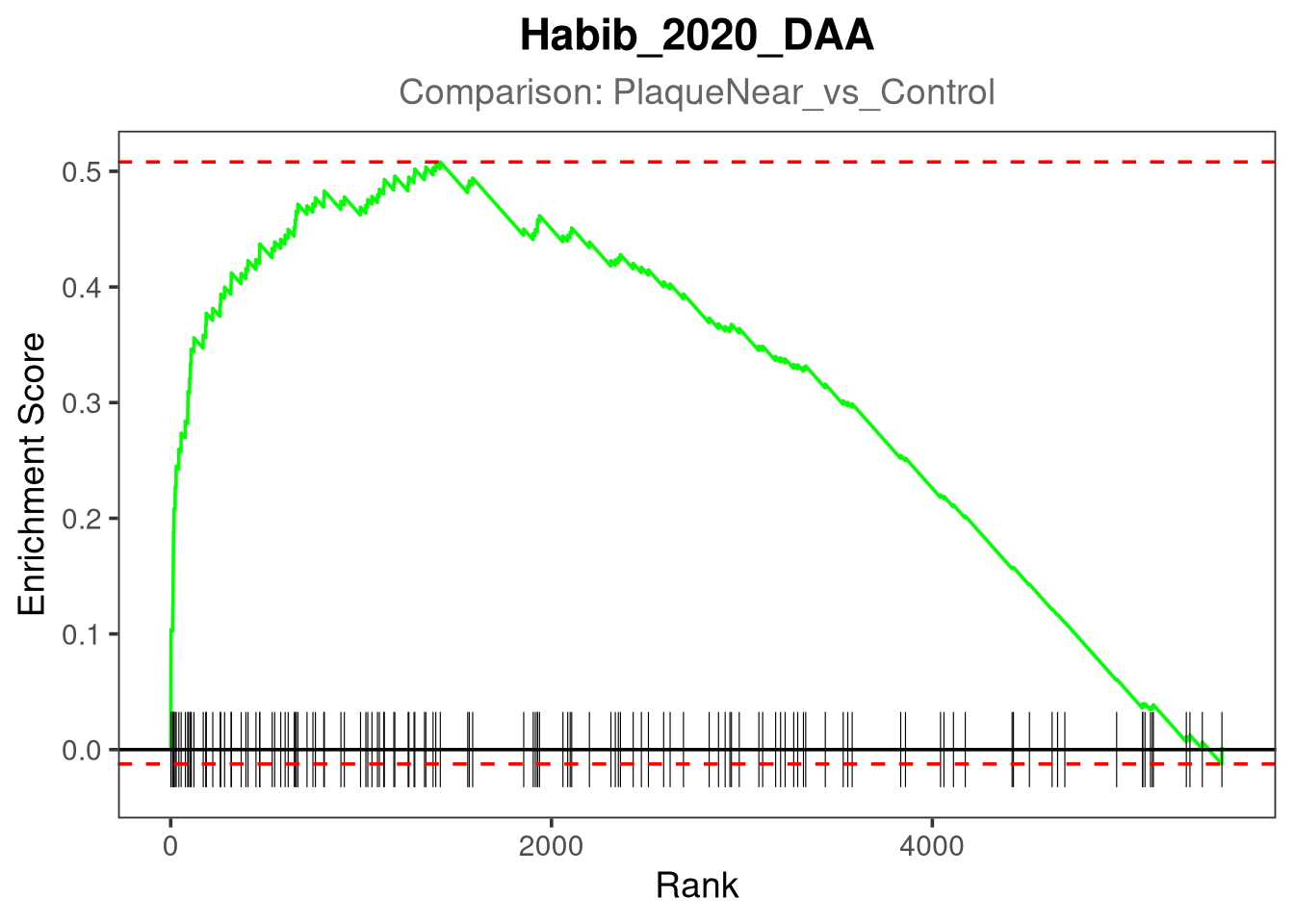
Plotting Habib_2020_DAA for PlaqueFar_vs_Control...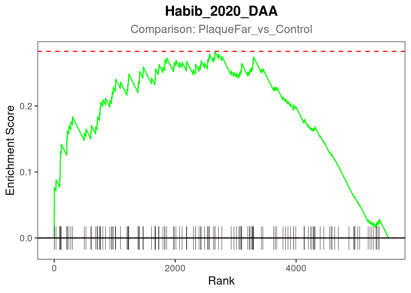
Plotting Habib_2020_DAA for PlaqueNear_vs_PlaqueFar...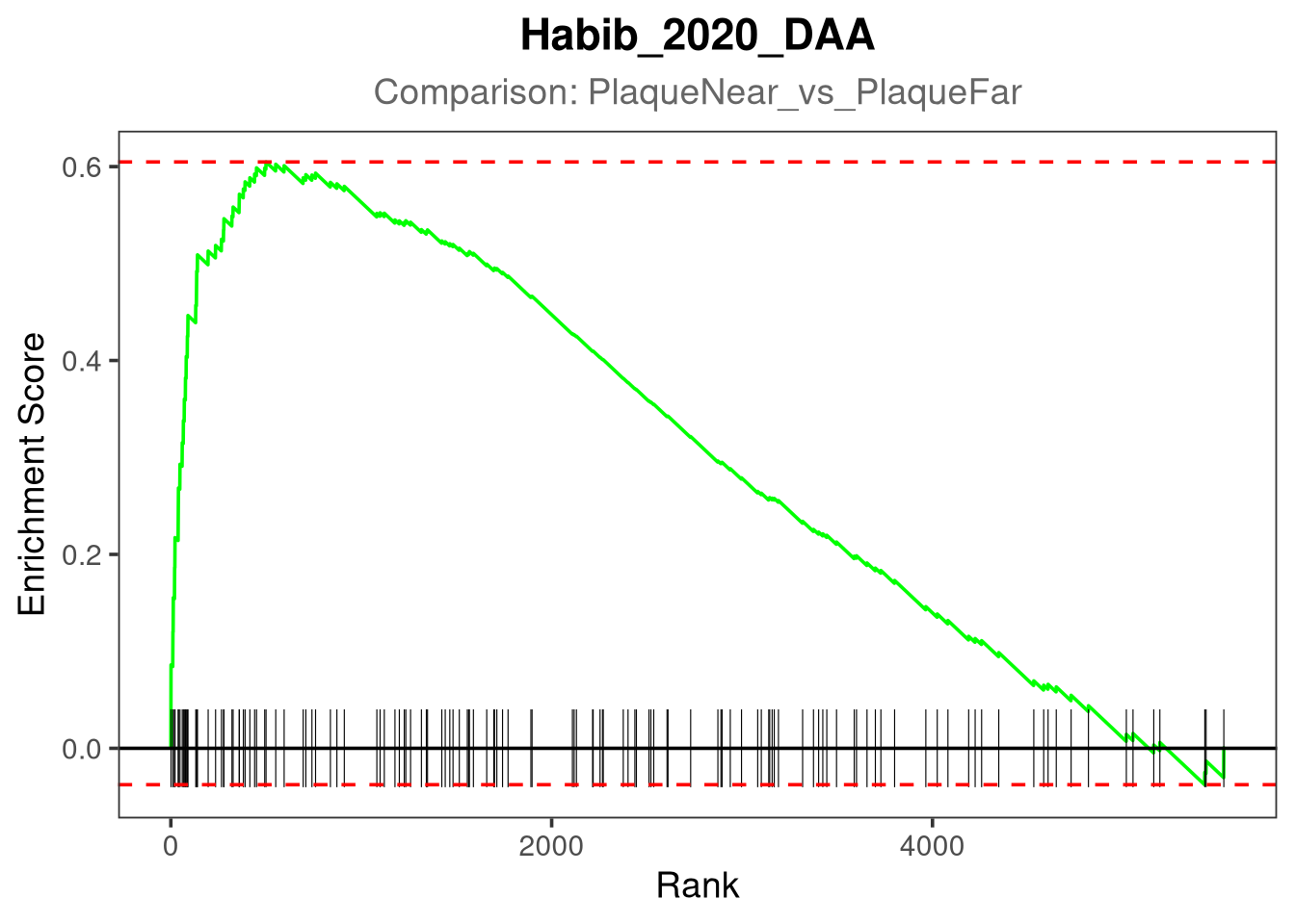
# Get top 10 upregulated proteins from PlaqueNear vs PlaqueFar
top10_near_vs_far <- comparisons_master[["PlaqueNear_vs_PlaqueFar"]] %>%
  sort(decreasing = TRUE) %>%
  head(10) %>%
  names()

# Get top 10 from Habib 2020 DAA signature
top10_habib <- head(daa_vector, 10)

# Define the background population
# Use all genes present in the rank list as the background
background_genes <- names(comparisons_master[["PlaqueNear_vs_PlaqueFar"]])
N <- length(background_genes)

# Calculate overlap
overlap <- intersect(top10_near_vs_far, top10_habib)
k <- length(overlap)  # observed overlap
m <- sum(top10_habib %in% background_genes)  # Habib top10 genes present in background
n <- N - m            # genes NOT in Habib top10
q <- length(top10_near_vs_far)  # size of your top10

# Hypergeometric test
# phyper(k-1) gives P(X >= k) i.e. probability of overlap >= observed by chance
p_val <- phyper(k - 1, m, n, q, lower.tail = FALSE)

cat("=== Hypergeometric Test: PlaqueNear vs PlaqueFar vs Habib 2020 DAA ===\n")
=== Hypergeometric Test: PlaqueNear vs PlaqueFar vs Habib 2020 DAA ===cat("Background (total detected proteins):", N, "\n")Background (total detected proteins): 5532 cat("Habib top 10 genes found in background:", m, "\n")Habib top 10 genes found in background: 6 cat("Your top 10 Near vs Far proteins:", q, "\n")Your top 10 Near vs Far proteins: 10 cat("Observed overlap:", k, "\n")Observed overlap: 1 cat("Overlapping genes:", paste(overlap, collapse = ", "), "\n")Overlapping genes: GFAP cat("P-value:", p_val, "\n\n")P-value: 0.01080195 # Visualise the overlap with a simple table
overlap_df <- data.frame(
Gene = background_genes,
In_Habib_Top10 = background_genes %in% top10_habib,
In_NearFar_Top10 = background_genes %in% top10_near_vs_far
) %>%
filter(In_Habib_Top10 | In_NearFar_Top10) %>%
mutate(
Overlap = In_Habib_Top10 & In_NearFar_Top10
) %>%
arrange(desc(Overlap))
print(overlap_df) Gene In_Habib_Top10 In_NearFar_Top10 Overlap
1 GFAP TRUE TRUE TRUE
2 NCOR1 FALSE TRUE FALSE
3 CLCN6 FALSE TRUE FALSE
4 DIDO1 FALSE TRUE FALSE
5 DPP7 FALSE TRUE FALSE
6 ARFGEF3 FALSE TRUE FALSE
7 SERPINC1 FALSE TRUE FALSE
8 ARL8B FALSE TRUE FALSE
9 ABCA3 FALSE TRUE FALSE
10 PTPN6 FALSE TRUE FALSE
11 APOE TRUE FALSE FALSE
12 CLU TRUE FALSE FALSE
13 CPE TRUE FALSE FALSE
14 CST3 TRUE FALSE FALSE
15 CD81 TRUE FALSE FALSE