1b: DAA marker check

Libraries

knitr::opts_knit$set(root.dir = '/nemo/lab/destrooperb/home/shared/zanettc/millie_proteomics')

library(data.table)
library(dplyr)

Attaching package: 'dplyr'

The following objects are masked from 'package:data.table':

    between, first, last

The following objects are masked from 'package:stats':

    filter, lag

The following objects are masked from 'package:base':

    intersect, setdiff, setequal, union

library(ggplot2)
library(tidyr)
library(stringr)
library(qs2)

qs2 0.1.6

Directories

base_dir <- "/nemo/lab/destrooperb/home/shared/zanettc/millie_proteomics"
run_num <- "run1"

# Pointing to where you saved the clean data, and where to output the plot
objects_dir <- file.path(base_dir, "data", "processed", run_num)
results_dir <- file.path(base_dir, "results", run_num)

Read in raw files

clean_meta <- fread(file.path(objects_dir, "clean_metadata.csv"))
clean_spec_raw <- fread(file.path(objects_dir, "clean_spec_raw.csv"))

Define function to calculate specific gene per condition, with the dot coloured by Batch

plot_target_genes <- function(genes_to_plot, raw_data, meta_data) {
  
  # 1. Subset raw data using regex pattern
  pattern <- paste(genes_to_plot, collapse="|")
  marker_raw <- raw_data[grepl(pattern, PG.Genes, ignore.case = TRUE)]
  
  if(nrow(marker_raw) == 0) {
    stop("None of the specified genes were found in the dataset.")
  }
  
  # 2. Pivot and clean
  marker_long <- marker_raw %>%
    select(PG.Genes, all_of(meta_data$Run)) %>%
    pivot_longer(cols = -PG.Genes, names_to = "Run", values_to = "Intensity") %>%
    # Extract the specific matched gene name for cleaner facet labels
    mutate(Marker = str_extract(PG.Genes, regex(pattern, ignore_case = TRUE))) %>%
    mutate(Marker = str_to_title(Marker)) %>% # Normalizes capitalization (e.g., gfap -> Gfap)
    mutate(Log2_Intensity = log2(Intensity + 1)) %>%
    mutate(Log2_Intensity = ifelse(Log2_Intensity == 0, NA, Log2_Intensity))
  
  # 3. Merge with metadata
  marker_plot_data <- merge(marker_long, meta_data, by = "Run")
  
  # 4. Generate Plot: Boxes = Condition, Dots = Batch
  p <- ggplot(marker_plot_data, aes(x = Condition, y = Log2_Intensity)) +
    # Boxplot colored by Condition
    geom_boxplot(aes(fill = Condition), outlier.shape = NA, alpha = 0.5) +
    # Jittered dots colored by Batch
    geom_jitter(aes(color = as.factor(Batch)), width = 0.2, size = 2, alpha = 0.8) +
    facet_wrap(~ Marker, scales = "free_y") +
    theme_minimal(base_size = 14) +
    # Reusing your established condition colors
    scale_fill_manual(values = c("control" = "#1b9e77", "plaque_near" = "#d95f02", "plaque_far" = "#7570b3")) +
    # High-contrast palette for the batch dots
    scale_color_brewer(palette = "Set1") +
    labs(
         x = "Biological Condition", 
         y = "Log2 Intensity", 
         fill = "Condition",
         color = "Batch") +
    theme(axis.text.x = element_text(angle = 45, hjust = 1, face = "bold"),
          strip.text = element_text(face = "bold", size = 14))
  
  return(p)
}

DAA markers are inverted to what would be expected for Batch 2 and 5

Indicates some sort of Batch mix up.

my_genes <- c("Gfap", "App", "Clu", "Apoe")

# Run the function
p_markers <- plot_target_genes(my_genes, clean_spec_raw, clean_meta)

# Display inline
print(p_markers)

Warning: Removed 672 rows containing non-finite outside the scale range
(`stat_boxplot()`).

Warning: Removed 672 rows containing missing values or values outside the scale range
(`geom_point()`).

marker_pdf_path <- file.path(results_dir, "Target_Genes_Check.pdf")
ggsave(marker_pdf_path, plot = p_markers, width = 10, height = 8)

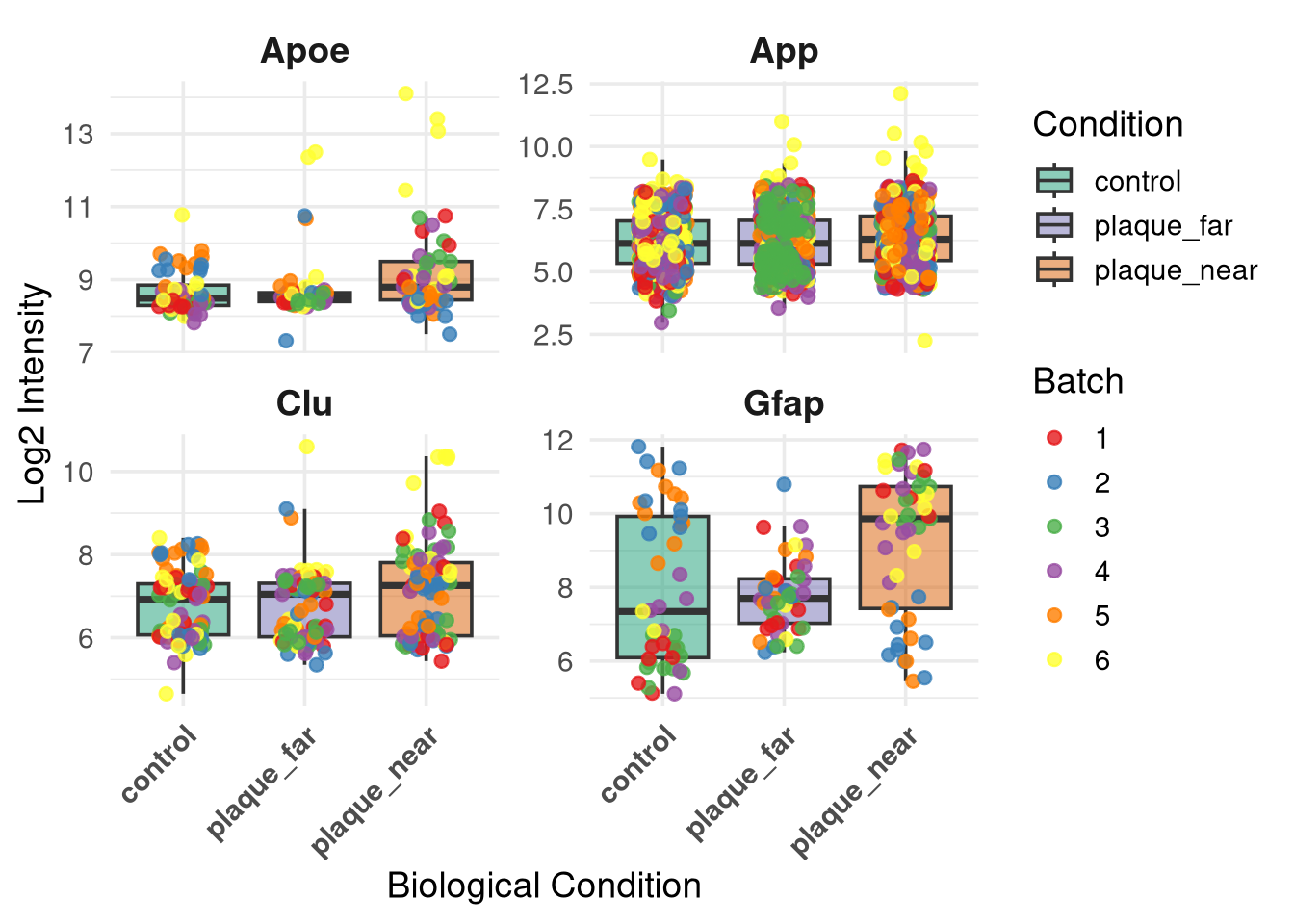
Warning: Removed 672 rows containing non-finite outside the scale range
(`stat_boxplot()`).
Removed 672 rows containing missing values or values outside the scale range
(`geom_point()`).

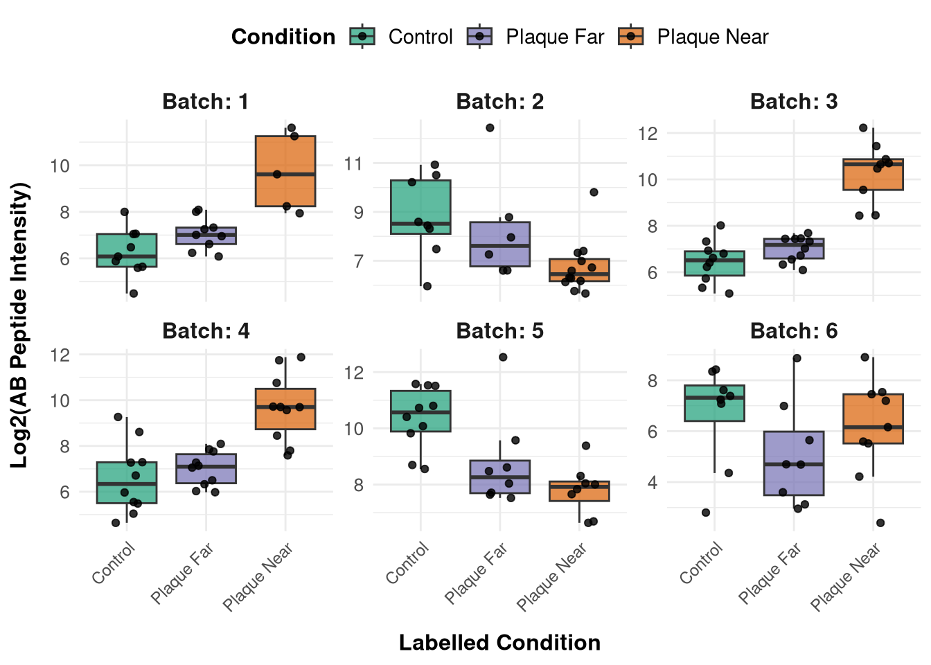
Pull in MSstats data to display Aß tryptic peptide plot

target_peptide <- "LVFFAEDVGSNK"

msstats_clean <- qs_read(file.path(objects_dir, "clean_msstats_input.qs2"))

colnames(msstats_clean)

 [1] "R.Condition"                  "R.FileName"                  
 [3] "R.Replicate"                  "PG.ProteinAccessions"        
 [5] "PG.ProteinGroups"             "PG.Qvalue"                   
 [7] "PG.Quantity"                  "PEP.GroupingKey"             
 [9] "PEP.StrippedSequence"         "PEP.Quantity"                
[11] "EG.iRTPredicted"              "EG.Library"                  
[13] "EG.ModifiedSequence"          "EG.PrecursorId"              
[15] "EG.Qvalue"                    "FG.Charge"                   
[17] "FG.Id"                        "FG.PrecMz"                   
[19] "FG.Quantity"                  "F.Charge"                    
[21] "F.FrgIon"                     "F.FrgLossType"               
[23] "F.FrgMz"                      "F.FrgNum"                    
[25] "F.FrgType"                    "F.ExcludedFromQuantification"
[27] "F.NormalizedPeakArea"         "F.NormalizedPeakHeight"      
[29] "F.PeakArea"                   "F.PeakHeight"                
[31] "Chip_location"                "Batch"                       
[33] "Condition"                    "BioReplicate"                

# Filter the cleaned MSstats data for the Aß peptide
ab_check_data <- msstats_clean %>%
  filter(PEP.StrippedSequence == target_peptide) %>%
  # Use F.PeakArea or F.NormalizedPeakArea for the raw intensity values
  group_by(R.FileName, Condition, Batch) %>%
  summarise(
    Total_Intensity = sum(F.PeakArea, na.rm = TRUE),
    .groups = "drop"
  ) %>%
  mutate(Log2_Intensity = log2(Total_Intensity + 1))


# 1. Clean up the data labels (Factor names)
ab_check_data$Condition <- factor(ab_check_data$Condition, 
                                  levels = c("control", "plaque_far", "plaque_near"),
                                  labels = c("Control", "Plaque Far", "Plaque Near"))

# 2. Update the plot
p_ab_check <- ggplot(ab_check_data, aes(x = Condition, y = Log2_Intensity, fill = Condition)) +
  geom_boxplot(outlier.shape = NA, alpha = 0.7) +
  geom_jitter(width = 0.2, alpha = 0.8) +
  facet_wrap(~ Batch, scales = "free_y", labeller = label_both) + 
  theme_minimal() +
  theme(
    legend.position = "top",
    legend.justification = "center",
    # Bold and larger Batch labels
    strip.text = element_text(face = "bold", size = 12),
    
    # Bold Axis Titles
    axis.title.x = element_text(face = "bold", size = 12, margin = margin(t = 10)),
    axis.title.y = element_text(face = "bold", size = 12, margin = margin(r = 10)),
    
    # Smaller, tilted X-axis labels to prevent overlap
    axis.text.x = element_text(size = 9, angle = 45, vjust = 1, hjust = 1),
    axis.text.y = element_text(size = 10),
    
    # Larger Legend
    legend.text = element_text(size = 11),
    legend.title = element_text(size = 12, face = "bold"),
    legend.key.size = unit(1.2, "lines"),
    
    # Remove plot title
    plot.title = element_blank()
  ) +
  # Map colors to the new "text-friendly" label names
  scale_fill_manual(values = c(
    "Control" = "#1b9e77", 
    "Plaque Far" = "#7570b3",
    "Plaque Near" = "#d95f02"
  )) +
  labs(
    x = "Labelled Condition",
    y = "Log2(AB Peptide Intensity)",
    fill = "Condition"
  )

print(p_ab_check)

# Save the plot
ggsave(file.path(results_dir, "AB_Peptide_Batch_Verification.pdf"), p_ab_check, width = 6, height = 6)